France - Large Domain Simulation

This second tutorial on smash aims to perform a simulation over the whole of metropolitan France with a simple model structure. The objective, compared to the first tutorial, is to create a mesh over a large spatial domain, to perform a forward run and to visualize the simulated discharge over the entire domain.

Required data

You need first to download all the required data.

Download

If the download was successful, a file named France-dataset.tar should be available. We can switch to the directory where this file has been downloaded and extract it using the following command:

tar xf France-dataset.tar

Now a folder called France-dataset should be accessible and contain the following files and folders:

• France_flwdir.tif

  A GeoTiff file containing the flow direction data,

• prcp

  A directory containing precipitation data in GeoTiff format with the following directory structure: %Y/%m/%d (2012/01/01),

• pet

  A directory containing daily interannual potential evapotranspiration data in GeoTiff format,

In this dataset, there are no gauge attributes or observed discharge, we are only interested in performing a forward run on a domain without optimization beforehand.

We can open a Python interface. The current working directory will be assumed to be the directory where the France-dataset is located.

Open a Python interface:

python3

Imports

We will first import everything we need in this tutorial. Both LogNorm and SymLogNorm will be used for plotting

In [1]: import smash

In [2]: import numpy as np

In [3]: import matplotlib.pyplot as plt

In [4]: from matplotlib.colors import LogNorm, SymLogNorm

Model creation

Model setup creation

The setup dictionary is pretty similar to the one used for the Cance tutorial except that we do not read observed discharge and the simulation period is different.

In [5]: setup = {
   ...:     "start_time": "2012-01-01 00:00",
   ...:     "end_time": "2012-01-02 08:00",
   ...:     "dt": 3_600,
   ...:     "hydrological_module": "gr4",
   ...:     "routing_module": "lr",
   ...:     "read_prcp": True,
   ...:     "prcp_conversion_factor": 0.1,
   ...:     "prcp_directory": "./France-dataset/prcp",
   ...:     "read_pet": True,
   ...:     "daily_interannual_pet": True,
   ...:     "pet_directory": "./France-dataset/pet",
   ...: }
   ...: 

Model mesh creation

For the mesh, we only need the flow direction file and the mainland France bounding box bbox to pass to the smash.factory.generate_mesh function. A bouding box in smash is a list of 4 values (xmin, xmax, ymin, ymax), each of which corresponds respectively to the x minimum value, the x maximum value, the y mimimum value and the y maximum value. The values must be in the same unit and projection as the flow direction.

In [6]: bbox = [100_000, 1_250_000, 6_050_000, 7_125_000] # Mainland Fance bbox in Lambert-93

In [7]: mesh = smash.factory.generate_mesh(
   ...:     flwdir_path="./France-dataset/France_flwdir.tif",
   ...:     bbox=bbox,
   ...: )
   ...: 

Note

Compare to a mesh generated with gauge attributes, the following variables are missing: flwdst, gauge_pos, code, area and area_dln.

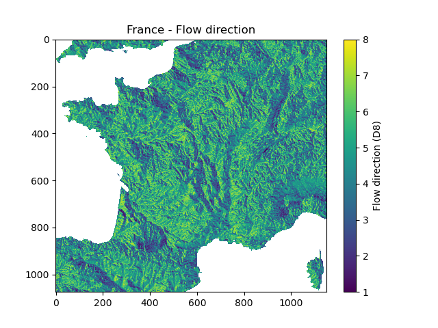
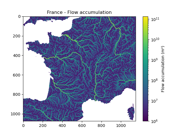
We can visualize the shape of the mesh, the flow direction and the flow accumulation

In [8]: mesh["nrow"], mesh["ncol"]
Out[8]: (1075, 1150)

In [9]: plt.imshow(mesh["flwdir"]);

In [10]: plt.colorbar(label="Flow direction (D8)");

In [11]: plt.title("France - Flow direction");

In [12]: plt.imshow(mesh["flwacc"], norm=LogNorm());

In [13]: plt.colorbar(label="Flow accumulation (m²)");

In [14]: plt.title("France - Flow accumulation");

Then, we can initialize the smash.Model object

In [15]: model = smash.Model(setup, mesh)
</> Computing mean atmospheric data
</> Adjusting GR interception capacity

Model simulation

Forward run

We can now call the Model.forward_run method, but by default and for memory reasons, the simulated discharge on the entire spatio-temporal domain is not saved. This means storing an numpy.ndarray of shape (nrow, ncol, ntime_step), which may be quite large depending on the simulation period and the spatial domain. To activate this option, the return_options argument must be filled in, specifying that you want to retrieve the simulated discharge on the whole domain. Whenever the return_options is filled in, the Model.forward_run method returns a smash.ForwardRun object storing these variables.

In [16]: fwd_run = model.forward_run(return_options={"q_domain": True})

In [17]: fwd_run
Out[17]: 
  q_domain: <class 'numpy.ndarray'>
 time_step: <class 'pandas.core.indexes.datetimes.DatetimeIndex'>

In [18]: fwd_run.time_step
Out[18]: 
DatetimeIndex(['2012-01-01 01:00:00', '2012-01-01 02:00:00',
               '2012-01-01 03:00:00', '2012-01-01 04:00:00',
               '2012-01-01 05:00:00', '2012-01-01 06:00:00',
               '2012-01-01 07:00:00', '2012-01-01 08:00:00',
               '2012-01-01 09:00:00', '2012-01-01 10:00:00',
               '2012-01-01 11:00:00', '2012-01-01 12:00:00',
               '2012-01-01 13:00:00', '2012-01-01 14:00:00',
               '2012-01-01 15:00:00', '2012-01-01 16:00:00',
               '2012-01-01 17:00:00', '2012-01-01 18:00:00',
               '2012-01-01 19:00:00', '2012-01-01 20:00:00',
               '2012-01-01 21:00:00', '2012-01-01 22:00:00',
               '2012-01-01 23:00:00', '2012-01-02 00:00:00',
               '2012-01-02 01:00:00', '2012-01-02 02:00:00',
               '2012-01-02 03:00:00', '2012-01-02 04:00:00',
               '2012-01-02 05:00:00', '2012-01-02 06:00:00',
               '2012-01-02 07:00:00', '2012-01-02 08:00:00'],
              dtype='datetime64[ns]', freq='3600s')

In [19]: fwd_run.q_domain.shape
Out[19]: (1075, 1150, 32)

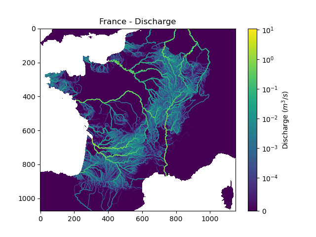
The returned object smash.ForwardRun contains two variables q_domain and time_step. With q_domain a numpy.ndarray of shape (nrow, ncol, ntime_step) storing the simulated discharge and time_step a pandas.DatetimeIndex storing the saved time steps. We can view the simulated discharge for one time step, for example the last one.

In [20]: q = fwd_run.q_domain[..., -1]

In [21]: q = np.where(model.mesh.active_cell == 0, np.nan, q) # Remove the non-active cells from the plot

In [22]: plt.imshow(q, norm=SymLogNorm(1e-4));

In [23]: plt.colorbar(label="Discharge $(m^3/s)$");

In [24]: plt.title("France - Discharge");

Note

Given that we performed a forward run on only 32 time steps with default rainfall-runoff parameters and initial states, the simulated discharge is not realistic.

By default, if the returned time steps are not defined, all the time steps are returned. It is possible to return only certain time steps by specifying them in the return_options argument, for example only the two last ones.

In [25]: time_step = ["2012-01-02 07:00", "2012-01-02 08:00"]

In [26]: fwd_run = model.forward_run(
   ....:     return_options={
   ....:         "time_step": time_step,
   ....:         "q_domain": True
   ....:     }
   ....: )
   ....: 

In [27]: fwd_run.time_step
Out[27]: DatetimeIndex(['2012-01-02 07:00:00', '2012-01-02 08:00:00'], dtype='datetime64[ns]', freq=None)

In [28]: fwd_run.q_domain.shape
Out[28]: (1075, 1150, 2)

In [29]: q = fwd_run.q_domain[..., -1]

In [30]: q = np.where(model.mesh.active_cell == 0, np.nan, q) # Remove the non-active cells from the plot

In [31]: plt.imshow(q, norm=SymLogNorm(1e-4));

In [32]: plt.colorbar(label="Discharge $(m^3/s)$");

In [33]: plt.title("France - Discharge");

This concludes this second tutorial on smash.