Forward & Inverse Problems#

This section explains:

The hydrological modeling problem (forward/direct problem), that consists in modeling the spatio-temporal evolution of water states-fluxes within a spatio-temporal domain given atmospheric forcings and basin physical descriptors.
The parameter estimation problem (inverse problem), that aims to estimating uncertain or unknows model parameters from the available spatio-temporal observations of hydrological state-fluxes and from basin physical descriptors.

Forward problem statement#

The forward/direct hydrological modeling problem statement is formulated here.

The 2D spatial domain is denoted $Ω$ with $x$ the vector of spatial coordinates, and $t$ is the time in the simulation window $] 0, T]$ .

Hydrological model definition#

The spatially distributed hydrological model is a dynamic operator $M$ projecting fields of atmospheric forcings $I$ , catchment physical descriptors $D$ onto surface discharge $Q$ , model states $h$ , and internal fluxes $q$ such that:

(1)#

U (x, t) = (Q, h, q) (x, t) = M ([I, D] (x, t); [θ, h_{0}] (x))

with $U (x, t)$ the modeled state-flux variables, $θ$ the parameters and $h_{0} = h (x, t = 0)$ the initial states.

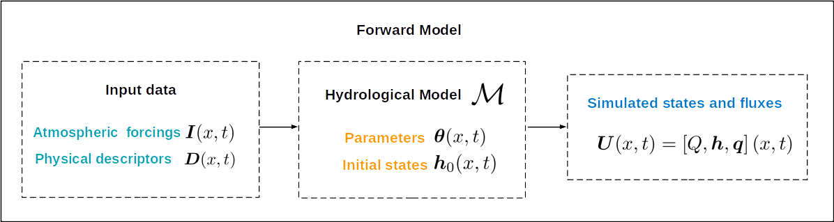
../_images/forward_simple_flowchart.png — Flowchart of the forward modeling problem: input data, forward hydrological model $M$ , simulated quantites.#

Operators Chaining Principle#

The forward hydrological model $M$ is obtained by chaining through fluxes at least two operators: the hydrological operator $M_{r r}$ to simulate runoff from atmospheric forcings and use this runoff to feed a routing operator $M_{h y}$ for cell to cell flow routing.

A snow module $M_{s n w}$ can also be added.

A learnable mapping $ϕ$ , composed of neural networks, can also be included into the forward model to predict parameters and/or fluxes corrections from various input data.

Several differentiable model structures are proposed in smash and detailed in model strucures section.

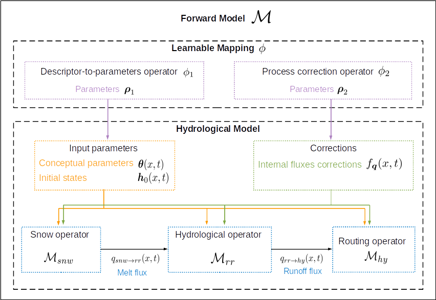
../_images/forward_composition_flowchart.png — Schematic view of operators composition into the forward model $M$ .#

Hydrological Model Operators#

The forward hydrological model is obtained by partial composition (each operator taking various other inputs data and paramters) of the flow operators writes:

(2)#

M = M_{h y} (., M_{r r} (., M_{s n w} (.)))

with the snow module $M_{s n w}$ producing a melt flux $q_{s n w \to r r} (x, t)$ feeding the production module $M_{r r}$ that produces runoff flux $q_{r r \to h y} (x, t)$ feeding the routing module $M_{h y}$ .

Models structures are detailed in model strucures section.

Learnable Mapping#

The spatio-temporal fields of model parameters and initial states can be constrained with spatialization rules (e.g. spatial patches for control reduction), or even explained by physiographic descriptors $D$ . This can be achieved via an operator $ϕ$ projecting physical descriptors $D$ onto model conceptual parameters such that

(3)#

(θ (x), h_{0} (x)) = ϕ (D (x, t), ρ)

with $ρ$ the control vector that can be optimized.

Consequently, replacing in Eq. 1 the parameters and initial states predicted by $ϕ$ operator, the forward model writes as:

(4)#

U (x, t) = (Q, h, q) (x, t) = M ([I, D] (x, t); ϕ (D (x, t), ρ))

The descriptors-to-parameters mappings are described in mapping section.

Parameter Estimation problem statement#

A general formulation of the model parameter estimation problem is given here. The aim is to fit modeled quantities $U (x, t) = (Q, h, q) (x, t)$ onto the available observations $Y^{*}$ of hydrological responses. This is for example the classical calibration problem on discharge time series at measurement gages over a river network, or more advanced data assimilation processes using multi source observations (ex. discharge, moisture, etc) and complex data-to-parameters mappings and other constrains and regularization.

A general description of the cost function, of the optimization problem and process is given here.

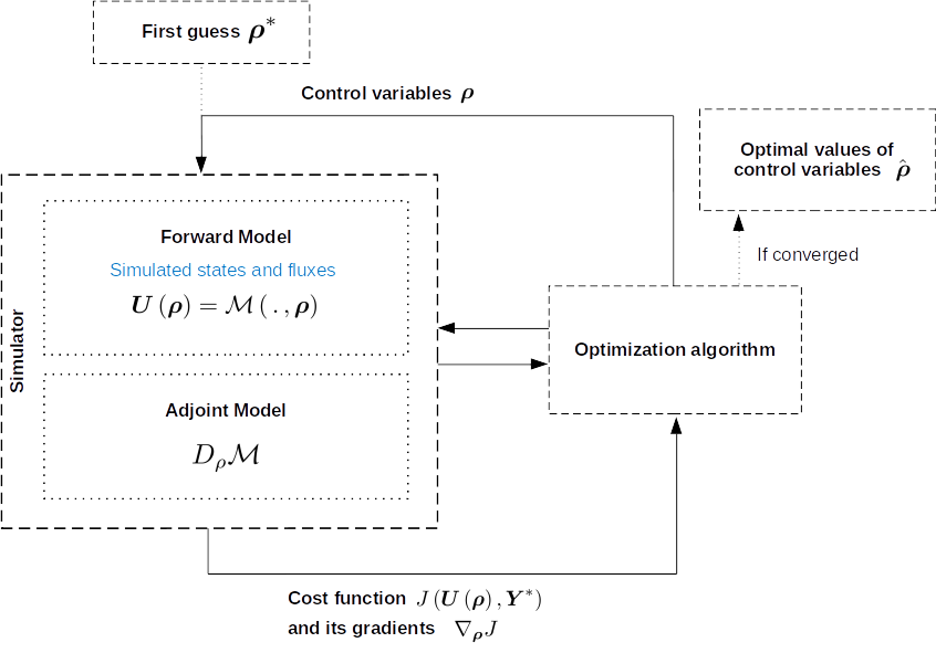
../_images/Inversion_process_flowchart.png — Schematic view of the optimization process of the parameters of the forward model $M$ (adapted from data assimilation course of [Monnier, 2024]). The parameters control vector $ρ$ that is optimized can simply be the hydrological model control $ρ := θ$ in case where the learnable mapping $ϕ$ is not used. This parameters control vector $ρ$ can also contain initial states $h_{0}$ (for example in short range data assimilation for states correction).#

Cost function#

Consider the following generic differentiable cost function composed of an observation term $J_{o b s}$ and a regularization term $J_{r e g}$ weighted by $α \geq 0$ :

(5)#

J = J_{o b s} + α J_{r e g}

Observation term#

The modeled states variables $U (x, t) = (Q, h, q) (x, t)$ are observed in a vector $Y = H [M (ρ)] \in Y$ with $H : X \mapsto Y$ the observation operator from state space $X$ to observation space $Y$ .

Given observations $Y^{*} (x^{*}, t^{*}) \in Y$ of hydrological responses over the domain $Ω \times] 0 . . T]$ , the model misfit to observations is measured through the observation cost function:

J_{o b s} = \frac{1}{2} {‖ Y - Y^{*} ‖}_{O}^{2}

(6)#

J_{o b s} (ρ) = \frac{1}{2} {‖ H [M (ρ)] - Y^{*} ‖}_{O}^{2}

with $O$ the observation error covariance matrix and the euclidian norm $‖ X ‖ O^{2} = X^{T} O X$

Regularization term#

The regularization term is for example a Thikhonov regularization that only involves the control $ρ$ and its background value $ρ^{*}$ from which optimization is started.

Optimization#

The optimization problem minimizing the misfit $J$ to observations writes as:

(7)#

\hat{ρ} = \underset{ρ}{argmin} J

This problem can be tackled with optimization algorithms adapted to high dimensional problems (L-BFGS-B [Zhu et al., 1994] or machine learning optimizers (e.g., Adam [Kingma and Ba, 2014])) that require the gradient $\nabla_{ρ} J$ of the cost function to the sought parameters $ρ$ . The computation of the cost gradient $\nabla_{ρ} J$ relies on the composed adjoint model $D_{ρ} M$ that is derived by automatic differenciation of the forward model, using the Tapenade software [Hascoet and Pascual, 2013]. The optimization is started from a first guess $ρ^{*}$ on the sought parameters $ρ$ .

Note

Following this general definition of the inverse problem, multiple definitions of observation cost function, regularization as well as mappings included into the forward model are possible with smash and detailled after along with several optimization algorithms taylored adapted to solve the different parameter optimization problems.