Lez - Regionalization#
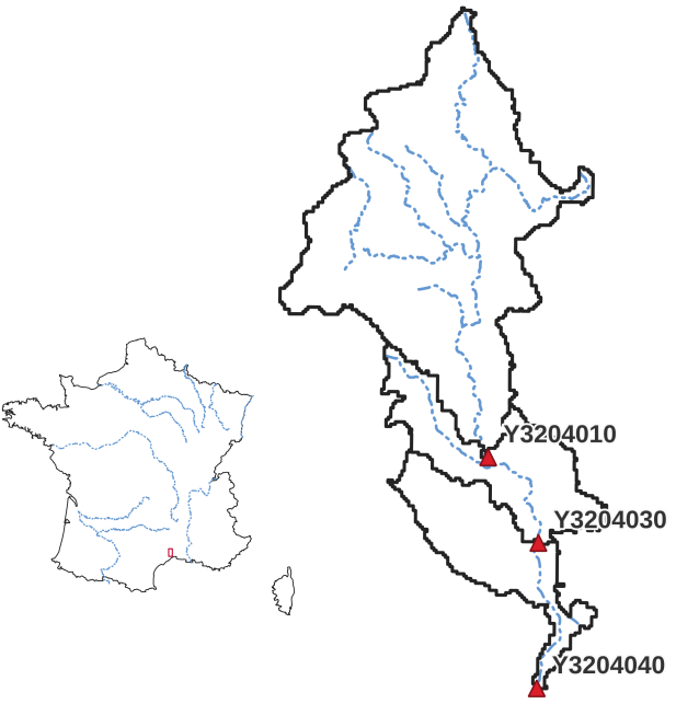
This guide on smash will be carried out on the French catchment, the Lez at Lattes and aims to perform an optimization of the
hydrological model considering regional mapping of physical descriptors onto model conceptual parameters.
The parameters \(\boldsymbol{\theta}\) can be written as a mapping \(\phi\) of descriptors \(\boldsymbol{\mathcal{D}}\)
(slope, drainage density, soil water storage, etc) and \(\boldsymbol{\rho}\) a control vector:
\(\boldsymbol{\theta}(x)=\phi\left(\boldsymbol{\mathcal{D}}(x),\boldsymbol{\rho}\right)\).
See the Mapping section for more details.
First, a shape is assumed for the mapping (here multi-polynomial or neural network). Then the control vector of the mapping needs to be optimized: \(\boldsymbol{\hat{\rho}}=\underset{\mathrm{\boldsymbol{\rho}}}{\text{argmin}}\;J\), with \(J\) the cost function.
Required data#
Hint
It is the same dataset as the Lez - Split Sample Test study, so possibly no need to re-download it.
You need first to download all the required data.
If the download was successful, a file named Lez-dataset.tar should be available. We can switch to the directory where this file has been
downloaded and extract it using the following command:
tar xf Lez-dataset.tar
Now a folder called Lez-dataset should be accessible and contain the following files and folders:
France_flwdir.tifA GeoTiff file containing the flow direction data,
gauge_attributes.csvA csv file containing the gauge attributes (gauge coordinates, drained area and code),
prcpA directory containing precipitation data in GeoTiff format with the following directory structure:
%Y/%m(2012/08),
petA directory containing daily interannual potential evapotranspiration data in GeoTiff format,
qobsA directory containing the observed discharge data in csv format,
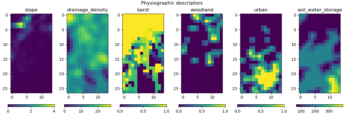
descriptorA directory containing physiographic descriptors in GeoTiff format.
Six physical descriptors are considered in this example, which are:
We can open a Python interface. The current working directory will be assumed to be the directory where
the Lez-dataset is located.
Open a Python interface:
python3
Imports#
We will first import everything we need in this tutorial.
In [1]: import smash

In [2]: import numpy as np

In [3]: import pandas as pd

In [4]: import matplotlib.pyplot as plt
Model creation#
Model setup creation#
In [5]: setup = {
   ...:     "start_time": "2012-08-01",
   ...:     "end_time": "2013-07-31",
   ...:     "dt": 86_400, # daily time step
   ...:     "hydrological_module": "gr4",
   ...:     "routing_module": "lr",
   ...:     "read_prcp": True,
   ...:     "prcp_directory": "./Lez-dataset/prcp",
   ...:     "read_pet": True,
   ...:     "pet_directory": "./Lez-dataset/pet",
   ...:     "read_qobs": True,
   ...:     "qobs_directory": "./Lez-dataset/qobs",
   ...:     "read_descriptor": True,
   ...:     "descriptor_directory": "./Lez-dataset/descriptor",
   ...:     "descriptor_name": [
   ...:         "slope",
   ...:         "drainage_density",
   ...:         "karst",
   ...:         "woodland",
   ...:         "urban",
   ...:         "soil_water_storage"
   ...:     ]
   ...: }
   ...:
Model mesh creation#
In [6]: gauge_attributes = pd.read_csv("./Lez-dataset/gauge_attributes.csv")

In [7]: mesh = smash.factory.generate_mesh(
   ...:     flwdir_path="./Lez-dataset/France_flwdir.tif",
   ...:     x=list(gauge_attributes["x"]),
   ...:     y=list(gauge_attributes["y"]),
   ...:     area=list(gauge_attributes["area"] * 1e6), # Convert km² to m²
   ...:     code=list(gauge_attributes["code"]),
   ...: )
   ...:
Then, we can initialize the smash.Model object
In [8]: model = smash.Model(setup, mesh)
</> Computing mean atmospheric data
Model simulation#
Multiple polynomial#
To optimize the rainfall-runoff model using a multiple polynomial mapping of descriptors to conceptual model parameters,
the value multi-polynomial simply needs to be passed to the mapping argument. We add another option to limit the number of iterations
by stopping the optimizer after 50 iterations.
In [9]: model_mp = smash.optimize(
   ...:     model,
   ...:     mapping="multi-polynomial",
   ...:     optimize_options={
   ...:         "termination_crit": dict(maxiter=50),
   ...:     },
   ...: )
   ...:
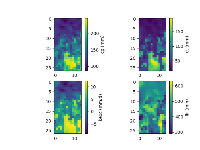
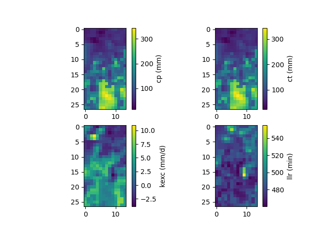
We have therefore optimized the set of rainfall-runoff parameters using a multiple polynomial regression constrained by physiographic descriptors. Here, most of the options used are the default ones, i.e. a minimization of one minus the Nash-Sutcliffe efficiency on the most downstream gauge of the domain. The resulting rainfall-runoff parameter maps can be viewed.
In [10]: f, ax = plt.subplots(2, 2)

In [11]: map_cp = ax[0,0].imshow(model_mp.get_rr_parameters("cp"));

In [12]: f.colorbar(map_cp, ax=ax[0,0], label="cp (mm)");

In [13]: map_ct = ax[0,1].imshow(model_mp.get_rr_parameters("ct"));

In [14]: f.colorbar(map_ct, ax=ax[0,1], label="ct (mm)");

In [15]: map_kexc = ax[1,0].imshow(model_mp.get_rr_parameters("kexc"));

In [16]: f.colorbar(map_kexc, ax=ax[1,0], label="kexc (mm/d)");

In [17]: map_llr = ax[1,1].imshow(model_mp.get_rr_parameters("llr"));

In [18]: f.colorbar(map_llr, ax=ax[1,1], label="llr (min)");
As well as performances at upstream gauges
In [19]: metrics = ["nse", "kge"]

In [20]: upstream_perf = pd.DataFrame(index=model.mesh.code[1:], columns=metrics)

In [21]: for m in metrics:
   ....:     upstream_perf[m] = np.round(smash.metrics(model_mp, metric=m)[1:], 2)
   ....:

In [22]: upstream_perf
Out[22]:
           nse   kge
Y3204030  0.79  0.63
Y3204010  0.60  0.68
Note
The two upstream gauges are the two last gauges of the list. This is why we use [1:] in the lists in order to take all the gauges
except the first, which is the downstream gauge on which the model has been calibrated.
Artificial neural network#
We can optimize the rainfall-runoff model using a neural network (NN) based mapping of descriptors to conceptual model parameters.
It is possible to define your own network to implement this optimization, but here we willl use the default neural network.
Similar to multiple polynomial mapping, all you have to do is to pass the value, ann to the mapping argument.
We also pass other options specific to the use of a NN:
optimize_optionsrandom_state: a random seed used to initialize neural network weights.learning_rate: the learning rate used for weights updates during training.termination_crit: the number of trainingepochsfor the neural network and a positive number to stop training when the loss function does not decrease below the current optimal value forearly_stoppingconsecutiveepochs
return_optionsnet: return the optimized neural network
In [23]: model_ann, opt_ann = smash.optimize(
   ....:     model,
   ....:     mapping="ann",
   ....:     optimize_options={
   ....:         "random_state": 23,
   ....:         "learning_rate": 0.004,
   ....:         "termination_crit": dict(epochs=100, early_stopping=20),
   ....:     },
   ....:     return_options={"net": True},
   ....: )
   ....:
Note
As we used the smash.optimize method (here an ADAM algorithm by default when choosing a NN based mapping) and asked for optional return values, this function will return two values, the optimized model
model_ann and the optional returns opt_ann.
Since we have returned the optimized neural network, we can visualize what it contains
In [24]: opt_ann.net
Out[24]:
+----------------------------------------------------------+
| Layer Type            Input/Output Shape  Num Parameters |
+----------------------------------------------------------+
| Dense                 (6,)/(21,)          147            |
| Activation (ReLU)     (21,)/(21,)         0              |
| Dense                 (21,)/(10,)         220            |
| Activation (ReLU)     (10,)/(10,)         0              |
| Dense                 (10,)/(4,)          44             |
| Activation (Sigmoid)  (4,)/(4,)           0              |
| Scale (MinMaxScale)   (4,)/(4,)           0              |
+----------------------------------------------------------+
Total parameters: 411
Trainable parameters: 411
The information displayed tells us that the default neural network is composed of 2 hidden dense layers followed by ReLU activation functions
and a final layer followed by a Sigmoid function. To scale the network output to the boundary condition, a MinMaxScale function is applied.
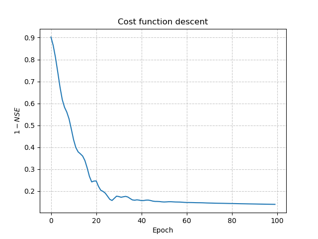
Other information is available in the smash.factory.Net object, including the value of the cost function at each iteration.
In [25]: plt.plot(opt_ann.net.history["loss_train"]);

In [26]: plt.xlabel("Epoch");

In [27]: plt.ylabel("$1-NSE$");

In [28]: plt.grid(alpha=.7, ls="--");

In [29]: plt.title("Cost function descent");
Finally, we can visualize parameters and performances
In [30]: f, ax = plt.subplots(2, 2)

In [31]: map_cp = ax[0,0].imshow(model_ann.get_rr_parameters("cp"));

In [32]: f.colorbar(map_cp, ax=ax[0,0], label="cp (mm)");

In [33]: map_ct = ax[0,1].imshow(model_ann.get_rr_parameters("ct"));

In [34]: f.colorbar(map_ct, ax=ax[0,1], label="ct (mm)");

In [35]: map_kexc = ax[1,0].imshow(model_ann.get_rr_parameters("kexc"));

In [36]: f.colorbar(map_kexc, ax=ax[1,0], label="kexc (mm/d)");

In [37]: map_llr = ax[1,1].imshow(model_ann.get_rr_parameters("llr"));

In [38]: f.colorbar(map_llr, ax=ax[1,1], label="llr (min)");
In [39]: metrics = ["nse", "kge"]

In [40]: upstream_perf = pd.DataFrame(index=model.mesh.code[1:], columns=metrics)

In [41]: for m in metrics:
   ....:     upstream_perf[m] = np.round(smash.metrics(model_ann, metric=m)[1:], 2)
   ....:

In [42]: upstream_perf
Out[42]:
           nse   kge
Y3204030  0.83  0.73
Y3204010  0.76  0.87