Cance - First Simulation

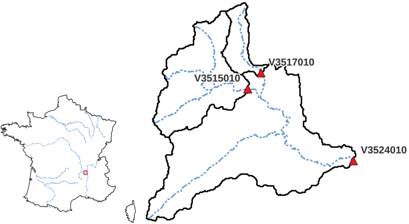
This first tutorial with smash will be carried out on a French catchment, the Cance at Sarras, a right bank tributary of the Rhône river. This catchment was chosen for this first tutorial because its moderate size (380 km²) enables fast computations at a spatial scale of 1km², and because it is well modeled with a low complexity approach. This tutorial aims to

• provide an overview of the input data required for modelling with smash,

• explain how to perform in Python a simulation and a simple model optimization from discharge data at a given gauging station.

Required data

Before you can start using smash, you need to download all the data required to run a simulation on this catchment.

Download

If the download was successful, a file named Cance-dataset.tar should be available. We can switch to the directory where this file has been downloaded and extract it using the following command:

tar xf Cance-dataset.tar

Now a folder called Cance-dataset should be accessible and contain the following files and folders for various spatio-temporal data:

• France_flwdir.tif

  A GeoTiff file containing the flow direction data,

• gauge_attributes.csv

  A csv file containing the gauge attributes (gauge coordinates, drainage area and code),

• prcp

  A directory containing precipitation data in GeoTiff format with the following directory structure: %Y/%m/%d (2014/09/15),

• pet

  A directory containing daily interannual potential evapotranspiration data in GeoTiff format,

• qobs

  A directory containing the observed discharge data in csv format.

Flow direction

The flow direction file is a mandatory input in order to create a mesh, its associated drainage plan \(\mathcal{D}_{\Omega}(x)\), and the localization on the mesh of the gauging stations that we want to model. Here, the France_flwdir.tif contains the flow direction data on the whole France, at a spatial resolution of 1km² using a Lambert-93 projection (EPSG: 2154). smash is using the following D8 convention for the flow direction.

Gauge attributes

To create a mesh containing information from the stations in addition to the flow direction file, gauge attributes are mandatory. The gauge attributes correspond to the spatial coordinates, the drainage area and the code of each gauge. The spatial coordinates must be in the same unit and projection as the flow direction file (meter and Lambert 93 respectively in our case), the drainage area in square meter (or square kilometer but it will need to be converted later). The gauge code can be any code that can be used to identify the station. The gauge_attributes.csv file has been filled in to provide this information for the 3 gauging stations of the Cance catchment.

Note

We don’t use the csv file directly in smash, we only use the data it contains. So it’s possible to store this data in another format as long as it can be read with Python.

Precipitation

Precipitation data is mandatory. smash expects a precipitation file per time step whose name contains a date in the following format %Y%m%d%H%M. The file must be in GeoTiff format at a resolution and projection identical to the flow direction file. Any unit can be chosen as long as it can be converted into a millimetre using a simple conversion factor (the unit used in this dataset is tenth of a millimetre). Regarding the structure of the precipitation folder, there is no strict rule, by default smash will fetch all the tif files in a folder provided by the user (i.e. prcp). However, when simulating a large number of time steps, we recommend sorting the files as much as possible to speed up access when reading those (ex. %Y/%m/%d, 2014/09/15).

Note

As you may have seen when opening any precipitation file, the data has already been cropped over the catchment area. This has been done simply to reduce the size of the files. It is possible to work with files whose spatial extent is different from the catchment area. smash will automatically crop to the correct area when the file is read.

Potential evapotranspiration

Potential evapotranspiration data is mandatory. The way in which potential evapotranspiration data is processed is identical to the precipitation. One difference to note is that instead of working with one potential evapotranspiration file per time step, it is possible to work with daily interannual data, which therefore requires a file per day whose name contains a date in the following format %m%d. Here, we provided daily interannual potential evapotranspiration data.

Observed discharge

Observed discharge is optional in case of simulation but mandatory in case of model calibration. smash expects a single-column csv file for each gauge whose name contains the gauge code provided in the gauge_attributes.csv file. The header of the column is the first time step of the time series, the data is the observed discharge in cubic meter per second and any negative value in the series will be interpreted as no-data.

Note

It is not necessary to restrict the observed discharge series to the simulation period. It is possible to provide a time series covering a larger time window over which smash will only read the lines corresponding to dates after the starting date provided in the header.

Now that a brief tour of the necessary data has been done, we can open a Python interface. The current working directory will be assumed to be the directory where the Cance-dataset is located.

Open a Python interface:

python3

Imports

We will first import everything we need in this tutorial: smash of course, the numerical computing library numpy, the data analysis and manipulation tool library pandas, and the visualization library matplotlib.

In [1]: import smash

In [2]: import numpy as np

In [3]: import pandas as pd

In [4]: import matplotlib.pyplot as plt

Hint

The visualization library matplotlib is not installed by default but can be installed with pip as follows:

pip install matplotlib

Model creation

The smash.Model object is the entity around which the whole smash package revolves. In order to initialize this object, two informations are necessary, the setup and the mesh.

Model setup creation

The setup is a Python dictionary (i.e. pairs of keys and values) which contains all information relating to the simulation period, the structure of the hydrological model and the reading of input data. For this first simulation let us create the following setup:

In [5]: setup = {
   ...:     "start_time": "2014-09-15 00:00",
   ...:     "end_time": "2014-11-14 00:00",
   ...:     "dt": 3_600,
   ...:     "hydrological_module": "gr4",
   ...:     "routing_module": "lr",
   ...:     "read_qobs": True,
   ...:     "qobs_directory": "./Cance-dataset/qobs",
   ...:     "read_prcp": True,
   ...:     "prcp_conversion_factor": 0.1,
   ...:     "prcp_directory": "./Cance-dataset/prcp",
   ...:     "read_pet": True,
   ...:     "daily_interannual_pet": True,
   ...:     "pet_directory": "./Cance-dataset/pet",
   ...: }
   ...: 

To get into more details, this setup is composed of:

• start_time

  The beginning of the simulation,

• end_time

  The end of the simulation,

• dt

  The simulation time step in second,

Note

The convention of smash is that start_time is the date used to initialize the model’s states. All the modeled state-flux variables (i.e. discharge, states, internal fluxes) will be computed over the period start_time + 1dt and end_time

• hydrological_module

  The hydrological module, to be chosen from [gr4, gr5, grd, loieau, vic3l],

  Hint

  See the Hydrological Module section

• routing_module

  The routing module, to be chosen from [lag0, lr, kw],

  Hint

  See the Routing Module section

• read_qobs

  Whether or not to read observed discharges files,

• qobs_directory

  The path to the observed discharges files,

• read_prcp

  Whether or not to read precipitation files,

• prcp_conversion_factor

  The precipitation conversion factor (the precipitation value in data, for example in \(1/10 mm\), will be multiplied by the conversion factor to reach precipitation in \(mm\) as needed by the hydrological modules),

• prcp_directory

  The path to the precipitation files,

• read_pet

  Whether or not to read potential evapotranspiration files,

• pet_conversion_factor

  The potential evapotranspiration conversion factor (the potential evapotranspiration value from data will be multiplied by the conversion factor to get \(mm\) as needed by the hydrological modules),

• daily_interannual_pet

  Whether or not to read potential evapotranspiration files as daily interannual value desaggregated to the corresponding time step dt,

• pet_directory

  The path to the potential evapotranspiration files,

In summary the current setup you defined above corresponds to :

• a simulation time window between 2014-09-15 00:00 and 2014-11-14 00:00 at an hourly time step.

• a hydrological model structure composed of the hydrological module gr4 applied on each pixel of the mesh and coupled to the routing module lr (linear reservoir) for conveying discharge from pixels to pixel downstream.

• input data of observed discharge, precipitation and potential evapotranspiration will be read from the directories defined in the setup and containing the previously downloaded case data. A few options have been added for some of the input data, the conversion factor for precipitation, given that our data is in tenths of a millimeter, and the information that we want to work with daily interannual potential evapotranspiration data.

Hint

Detailed information on the model setup can be obtained from the API reference section of smash.Model.

Model mesh creation

Once the setup has been created, we can move on to the mesh creation. The mesh is also a Python dictionary but it is automatically generated with the smash.factory.generate_mesh function. To run this function, we need to pass the path of the flow direction file France_flwdir.tif as well as the data stored in the csv file gauge_attrivutes.csv.

In [6]: gauge_attributes = pd.read_csv("./Cance-dataset/gauge_attributes.csv")

In [7]: mesh = smash.factory.generate_mesh(
   ...:     flwdir_path="./Cance-dataset/France_flwdir.tif",
   ...:     x=list(gauge_attributes["x"]),
   ...:     y=list(gauge_attributes["y"]),
   ...:     area=list(gauge_attributes["area"] * 1e6), # Convert km² to m²
   ...:     code=list(gauge_attributes["code"]),
   ...: )
   ...: 

Note

We could also have passed on the gauge attributes directly without a csv file.

In [8]: mesh = smash.factory.generate_mesh(
   ...:     flwdir_path="./Cance-dataset/France_flwdir.tif",
   ...:     x=[840_261, 826_553, 828_269],
   ...:     y=[6_457_807, 6_467_115, 6_469_198],
   ...:     area=[381.7 * 1e6, 107 * 1e6, 25.3 * 1e6], # Convert km² to m²
   ...:     code=["V3524010", "V3515010", "V3517010"],
   ...: )
   ...: 

In [9]: mesh.keys()
Out[9]: dict_keys(['xres', 'yres', 'xmin', 'ymax', 'nrow', 'ncol', 'dx', 'dy', 'flwdir', 'flwdst', 'flwacc', 'npar', 'ncpar', 'cscpar', 'cpar_to_rowcol', 'flwpar', 'nac', 'active_cell', 'ng', 'gauge_pos', 'code', 'area', 'area_dln'])

To get into more details, this mesh is composed of:

• xres, yres

  The spatial resolution (unit of the flow directions map, meter)

  In [10]: mesh["xres"], mesh["yres"]
  Out[10]: (1000.0, 1000.0)
  

• xmin, ymax

  The coordinates of the upper left corner (unit of the flow directions map, meter)

  In [11]: mesh["xmin"], mesh["ymax"]
  Out[11]: (np.float64(813000.0), np.float64(6478000.0))
  

• nrow, ncol

  The number of rows and columns

  In [12]: mesh["nrow"], mesh["ncol"]
  Out[12]: (28, 28)
  

• dx, dy

  The spatial step in meter. These variables are arrays of shape (nrow, ncol). In this study, the mesh is a regular grid with a constant spatial step defining squared cells.

  In [13]: mesh["dx"][0,0], mesh["dy"][0,0]
  Out[13]: (np.float32(1000.0), np.float32(1000.0))
  

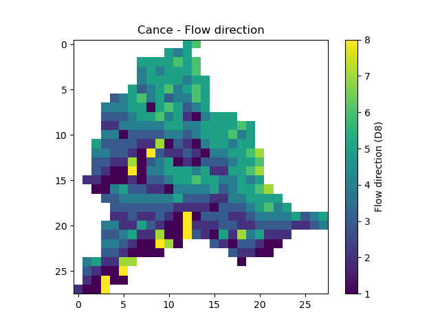
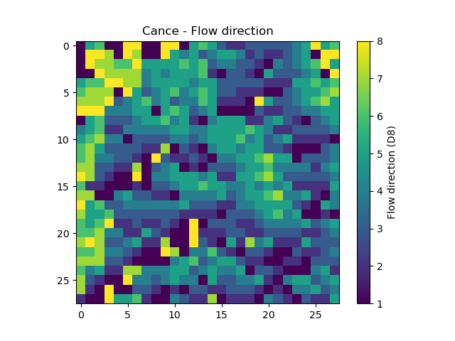
• flwdir

  The flow direction that can be simply visualized that way

  In [14]: plt.imshow(mesh["flwdir"]);
  
  In [15]: plt.colorbar(label="Flow direction (D8)");
  
  In [16]: plt.title("Cance - Flow direction");
  

  

Hint

If the plot is not displayed, try the plt.show() command.

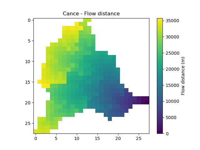
• flwdst

  The flow distance in meter from the most downstream outlet

  In [17]: plt.imshow(mesh["flwdst"]);
  
  In [18]: plt.colorbar(label="Flow distance (m)");
  
  In [19]: plt.title("Cance - Flow distance");
  

  

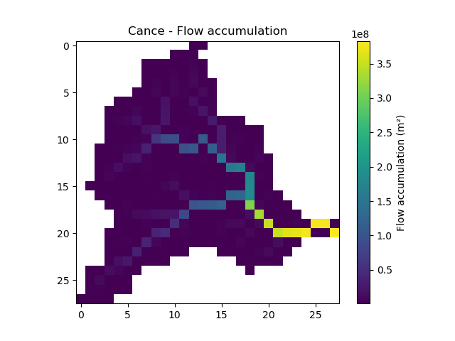
• flwacc

  The flow accumulation in square meter

  In [20]: plt.imshow(mesh["flwacc"]);
  
  In [21]: plt.colorbar(label="Flow accumulation (m²)");
  
  In [22]: plt.title("Cance - Flow accumulation");
  

  

• npar, ncpar, cscpar, cpar_to_rowcol, flwpar

  All the variables related to independent routing partitions. We won’t go into too much detail about these variables, as they simply allow us, in parallel computation, to identify which are the independent cells in the drainage network.

  In [23]: mesh["npar"], mesh["ncpar"], mesh["cscpar"], mesh["cpar_to_rowcol"]
  Out[23]: 
  (np.int32(31),
   array([408, 145,  67,  36,  23,  16,  13,  10,   6,   6,   5,   5,   4,
            4,   4,   4,   4,   4,   3,   3,   3,   2,   1,   1,   1,   1,
            1,   1,   1,   1,   1], dtype=int32),
   array([  0, 408, 553, 620, 656, 679, 695, 708, 718, 724, 730, 735, 740,
          744, 748, 752, 756, 760, 764, 767, 770, 773, 775, 776, 777, 778,
          779, 780, 781, 782, 783], dtype=int32),
   array([[ 3,  0],
          [ 4,  0],
          [ 8,  0],
          ...,
          [19, 25],
          [19, 26],
          [20, 27]], dtype=int32))
  
  In [24]: plt.imshow(mesh["flwpar"]);
  
  In [25]: plt.colorbar(label="Flow partition (-)");
  
  In [26]: plt.title("Cance - Flow partition");
  

  

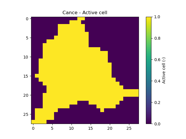
• nac, active_cell

  The number of active cells, nac and the mask of active cells, active_cell. When meshing, we define a rectangular area of shape (nrow, ncol) in which only a certain number of cells contribute to the discharge at the mesh gauges. This saves us computing time and memory.

  In [27]: mesh["nac"]
  Out[27]: 383
  
  In [28]: plt.imshow(mesh["active_cell"]);
  
  In [29]: plt.colorbar(label="Active cell (-)");
  
  In [30]: plt.title("Cance - Active cell");
  

  

• ng, gauge_pos, code, area, area_dln

  All the variables related to the gauges. The number of gauges, ng, the gauges position in terms of rows and columns, gauge_pos, the gauges code, code, the “real” drainage area, area and the delineated drainage area, area_dln.

  In [31]: mesh["ng"], mesh["gauge_pos"], mesh["code"], mesh["area"], mesh["area_dln"]
  Out[31]: 
  (3,
   array([[20, 27],
          [10, 13],
          [ 8, 14]], dtype=int32),
   array(['V3524010', 'V3515010', 'V3517010'], dtype='<U8'),
   array([3.817e+08, 1.070e+08, 2.530e+07], dtype=float32),
   array([3.83e+08, 1.08e+08, 2.80e+07], dtype=float32))
  

An important step after generating the mesh is to check that the stations have been correctly placed on the flow direction map. To do this, we can try to visualize on which cell each station is located and whether the delineated drainage area is close to the “real” drainage area entered.

In [32]: base = np.zeros(shape=(mesh["nrow"], mesh["ncol"]))

In [33]: base = np.where(mesh["active_cell"] == 0, np.nan, base)

In [34]: for pos in mesh["gauge_pos"]:
   ....:     base[pos[0], pos[1]] = 1
   ....: 

In [35]: plt.imshow(base, cmap="Set1_r");

In [36]: plt.title("Cance - Gauge position");

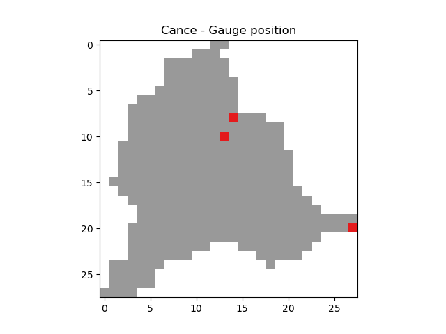
In [37]: (mesh["area"] - mesh["area_dln"]) / mesh["area"] * 100 # Relative error in %
Out[37]: array([ -0.34058163,  -0.93457943, -10.671937  ], dtype=float32)

For this mesh, we have a negative relative error on the simulated drainage area that varies from -0.3% for the most downstream gauge to -10% for the most upstream one (which can be explained by the fact that small upstream catchments are more sensitive to the relatively coarse mesh resolution).

Save setup and mesh

Before constructing the smash.Model object, we can save (serialize) the setup and the mesh to avoid having to do it every time you want to run a simulation on the same case, with the two following functions, smash.io.save_setup and smash.io.save_mesh. It will save the setup in YAML format and the mesh in HDF5 format.

In [38]: smash.io.save_setup(setup, "setup.yaml")

In [39]: smash.io.save_mesh(mesh, "mesh.hdf5")

Note

The setup and mesh can be read back with the smash.io.read_setup and smash.io.read_mesh functions

In [40]: setup = smash.io.read_setup("setup.yaml")

In [41]: mesh = smash.io.read_mesh("mesh.hdf5")

Finally, initialize the smash.Model object

In [42]: model = smash.Model(setup, mesh)
</> Computing mean atmospheric data
</> Adjusting GR interception capacity

In [43]: model
Out[43]: 
Model
    atmos_data: ['mean_pet', 'mean_prcp', '...', 'sparse_prcp', 'sparse_snow']
    mesh: ['active_cell', 'area', '...', 'xres', 'ymax']
    physio_data: ['descriptor', 'l_descriptor', 'u_descriptor']
    response: ['q']
    response_data: ['q']
    rr_final_states: ['keys', 'values']
    rr_initial_states: ['keys', 'values']
    rr_parameters: ['keys', 'values']
    serr_mu_parameters: ['keys', 'values']
    serr_sigma_parameters: ['keys', 'values']
    setup: ['adjust_interception', 'compute_mean_atmos', '...', 'temp_access', 'temp_directory']
    u_response_data: ['q_stdev']

Model attributes

The smash.Model object is a complex structure with several attributes and associated methods. Not all of these will be detailed in this tutorial. As you can see by displaying the smash.Model object above after initializing it, several attributes are accessible:

Setup

Model.setup contains all the information previously passed through the setup dictionary plus a set of other variables filled in by default or potentially not used afterwards.

In [44]: model.setup.start_time, model.setup.end_time, model.setup.dt
Out[44]: ('2014-09-15 00:00', '2014-11-14 00:00', 3600.0)

Mesh

Model.mesh contains all the information previously passed through the mesh dictionary.

In [45]: model.mesh.nrow, model.mesh.ncol, model.mesh.nac
Out[45]: (28, 28, 383)

In [46]: plt.imshow(model.mesh.flwdir);

In [47]: plt.colorbar(label="Flow direction (D8)");

In [48]: plt.title("Cance - Flow direction");

Note

Once the smash.Model object is initialized, the numpy.ndarray of the mesh are not masked anymore in the Model.mesh. It is therefore normal to have a difference in the non-active cells.

Atmospheric data

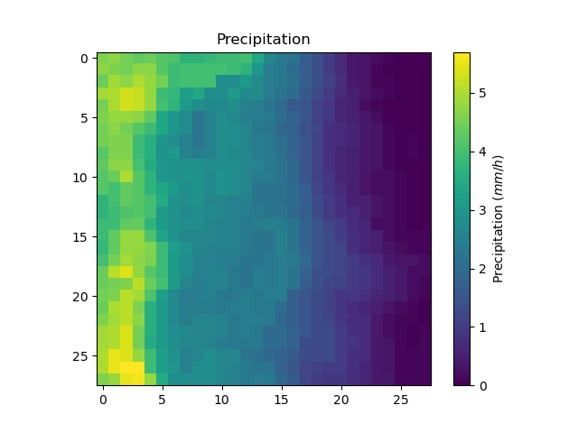
Model.atmos_data contains all the atmospheric data, here precipitation (prcp) and potential evapotranspiration (pet) that are stored as numpy.ndarray of shape (nrow, ncol, ntime_step) (one 2D array per time step). We can visualize the value of precipitation for an arbitrary time step.

In [49]: plt.imshow(model.atmos_data.prcp[..., 1200]);

In [50]: plt.colorbar(label="Precipitation ($mm/h$)");

In [51]: plt.title("Precipitation");

Or masked on the active cells of the catchment

In [52]: ma_prcp = np.where(
   ....:     model.mesh.active_cell == 0,
   ....:     np.nan,
   ....:     model.atmos_data.prcp[..., 1200]
   ....: )
   ....: 

In [53]: plt.imshow(ma_prcp);

In [54]: plt.colorbar(label="Precipitation ($mm/h$)");

In [55]: plt.title("Masked precipitation");

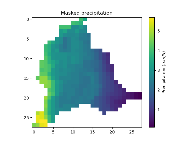
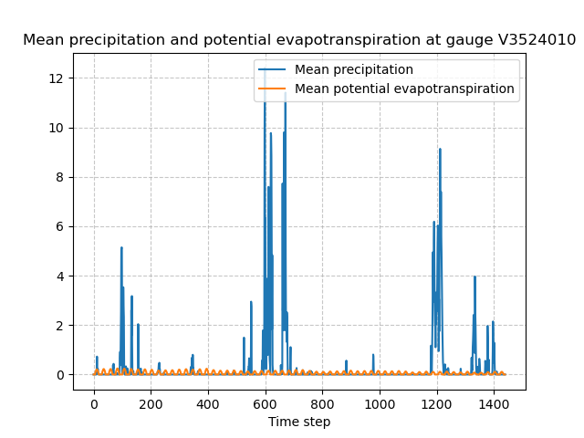
The spatial average of precipitation (mean_prcp) and potential evapotranspiration (mean_pet) over each gauge are also computed and stored in Model.atmos_data. They are numpy.ndarray of shape (ng, ntime_step), one temporal series by gauge.

In [56]: code = model.mesh.code[0]

In [57]: plt.plot(model.atmos_data.mean_prcp[0, :], label="Mean precipitation");

In [58]: plt.plot(model.atmos_data.mean_pet[0, :], label="Mean potential evapotranspiration");

In [59]: plt.grid(ls="--", alpha=.7);

In [60]: plt.legend();

In [61]: plt.xlabel("Time step");

In [62]: plt.title(
   ....:     f"Mean precipitation and potential evapotranspiration at gauge {code}"
   ....: );
   ....: 

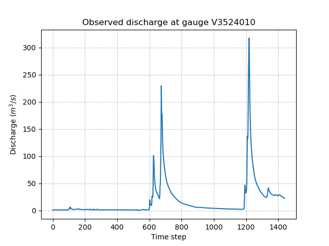
Response data

Model.response_data contains all the model response data. Currently, the only model response data is the observed discharge (q). The observed discharge is a numpy.ndarray of shape (ng, ntime_step), one temporal series by gauge.

In [63]: code = model.mesh.code[0]

In [64]: plt.plot(model.response_data.q[0, :]);

In [65]: plt.grid(ls="--", alpha=.7);

In [66]: plt.xlabel("Time step");

In [67]: plt.ylabel("Discharge ($m^3/s$)")
Out[67]: Text(0, 0.5, 'Discharge ($m^3/s$)')

In [68]: plt.title(
   ....:     f"Observed discharge at gauge {code}"
   ....: );
   ....: 

Rainfall-runoff parameters

Model.rr_parameters contains all the rainfall-runoff parameters. The rainfall-runoff parameters available depend on the chosen model structure and of the different modules that compose it. Here, we have selected the hydrological module gr4 and the routing module lr. This attribute consists of one variable storing the keys i.e. the names of the rainfall-runoff parameters and another storing their values, a numpy.ndarray of shape (nrow, ncol, nrrp), where nrrp is the number of rainfall-runoff parameters available.

In [69]: model.setup.nrrp, model.rr_parameters.keys
Out[69]: (5, array(['ci', 'cp', 'ct', 'kexc', 'llr'], dtype='<U128'))

To access the values of a specific rainfall-runoff parameter, it is possible to use the Model.get_rr_parameters method, here applied to get the spatial values of the production reservoir capacity

In [70]: model.get_rr_parameters("cp")[:10, :10] # Avoid printing all the cells
Out[70]: 
array([[200., 200., 200., 200., 200., 200., 200., 200., 200., 200.],
       [200., 200., 200., 200., 200., 200., 200., 200., 200., 200.],
       [200., 200., 200., 200., 200., 200., 200., 200., 200., 200.],
       [200., 200., 200., 200., 200., 200., 200., 200., 200., 200.],
       [200., 200., 200., 200., 200., 200., 200., 200., 200., 200.],
       [200., 200., 200., 200., 200., 200., 200., 200., 200., 200.],
       [200., 200., 200., 200., 200., 200., 200., 200., 200., 200.],
       [200., 200., 200., 200., 200., 200., 200., 200., 200., 200.],
       [200., 200., 200., 200., 200., 200., 200., 200., 200., 200.],
       [200., 200., 200., 200., 200., 200., 200., 200., 200., 200.]],
      dtype=float32)

The rainfall-runoff parameters are filled in with default spatially uniform values but can be modified using the Model.set_rr_parameters

In [71]: model.set_rr_parameters("cp", 134)

In [72]: model.get_rr_parameters("cp")[:10, :10]
Out[72]: 
array([[134., 134., 134., 134., 134., 134., 134., 134., 134., 134.],
       [134., 134., 134., 134., 134., 134., 134., 134., 134., 134.],
       [134., 134., 134., 134., 134., 134., 134., 134., 134., 134.],
       [134., 134., 134., 134., 134., 134., 134., 134., 134., 134.],
       [134., 134., 134., 134., 134., 134., 134., 134., 134., 134.],
       [134., 134., 134., 134., 134., 134., 134., 134., 134., 134.],
       [134., 134., 134., 134., 134., 134., 134., 134., 134., 134.],
       [134., 134., 134., 134., 134., 134., 134., 134., 134., 134.],
       [134., 134., 134., 134., 134., 134., 134., 134., 134., 134.],
       [134., 134., 134., 134., 134., 134., 134., 134., 134., 134.]],
      dtype=float32)

In [73]: model.set_rr_parameters("cp", 200) # Set the default value back

Rainfall-runoff initial states

Model.rr_initial_states contains all the rainfall-runoff initial states. This attribute is very similar to the rainfall-runoff parameters, both in its construction and in the variables it contains.

In [74]: model.setup.nrrs, model.rr_initial_states.keys
Out[74]: (4, array(['hi', 'hp', 'ht', 'hlr'], dtype='<U128'))

Methods similar to those used for rainfall-runoff parameters are available for states

In [75]: model.get_rr_initial_states("hp")[:10, :10]
Out[75]: 
array([[0.01, 0.01, 0.01, 0.01, 0.01, 0.01, 0.01, 0.01, 0.01, 0.01],
       [0.01, 0.01, 0.01, 0.01, 0.01, 0.01, 0.01, 0.01, 0.01, 0.01],
       [0.01, 0.01, 0.01, 0.01, 0.01, 0.01, 0.01, 0.01, 0.01, 0.01],
       [0.01, 0.01, 0.01, 0.01, 0.01, 0.01, 0.01, 0.01, 0.01, 0.01],
       [0.01, 0.01, 0.01, 0.01, 0.01, 0.01, 0.01, 0.01, 0.01, 0.01],
       [0.01, 0.01, 0.01, 0.01, 0.01, 0.01, 0.01, 0.01, 0.01, 0.01],
       [0.01, 0.01, 0.01, 0.01, 0.01, 0.01, 0.01, 0.01, 0.01, 0.01],
       [0.01, 0.01, 0.01, 0.01, 0.01, 0.01, 0.01, 0.01, 0.01, 0.01],
       [0.01, 0.01, 0.01, 0.01, 0.01, 0.01, 0.01, 0.01, 0.01, 0.01],
       [0.01, 0.01, 0.01, 0.01, 0.01, 0.01, 0.01, 0.01, 0.01, 0.01]],
      dtype=float32)

In [76]: model.set_rr_initial_states("hp", 0.23)

In [77]: model.get_rr_initial_states("hp")[:10, :10]
Out[77]: 
array([[0.23, 0.23, 0.23, 0.23, 0.23, 0.23, 0.23, 0.23, 0.23, 0.23],
       [0.23, 0.23, 0.23, 0.23, 0.23, 0.23, 0.23, 0.23, 0.23, 0.23],
       [0.23, 0.23, 0.23, 0.23, 0.23, 0.23, 0.23, 0.23, 0.23, 0.23],
       [0.23, 0.23, 0.23, 0.23, 0.23, 0.23, 0.23, 0.23, 0.23, 0.23],
       [0.23, 0.23, 0.23, 0.23, 0.23, 0.23, 0.23, 0.23, 0.23, 0.23],
       [0.23, 0.23, 0.23, 0.23, 0.23, 0.23, 0.23, 0.23, 0.23, 0.23],
       [0.23, 0.23, 0.23, 0.23, 0.23, 0.23, 0.23, 0.23, 0.23, 0.23],
       [0.23, 0.23, 0.23, 0.23, 0.23, 0.23, 0.23, 0.23, 0.23, 0.23],
       [0.23, 0.23, 0.23, 0.23, 0.23, 0.23, 0.23, 0.23, 0.23, 0.23],
       [0.23, 0.23, 0.23, 0.23, 0.23, 0.23, 0.23, 0.23, 0.23, 0.23]],
      dtype=float32)

In [78]: model.set_rr_initial_states("hp", 0.01) # Set the default value back

Rainfall-runoff final states

Model.rr_final_states contains all the rainfall-runoff final states, i.e. at the end of the simulation time window defined in setup. This attribute is identical to the rainfall-runoff initial states but for final ones. The final states are updated once a simulation is performed.

In [79]: model.setup.nrrs, model.rr_final_states.keys
Out[79]: (4, array(['hi', 'hp', 'ht', 'hlr'], dtype='<U128'))

Rainfall-runoff final states only have getters and are by default filled in with -99 until a simulation has been performed.

In [80]: model.get_rr_final_states("hp")[:10, :10]
Out[80]: 
array([[-99., -99., -99., -99., -99., -99., -99., -99., -99., -99.],
       [-99., -99., -99., -99., -99., -99., -99., -99., -99., -99.],
       [-99., -99., -99., -99., -99., -99., -99., -99., -99., -99.],
       [-99., -99., -99., -99., -99., -99., -99., -99., -99., -99.],
       [-99., -99., -99., -99., -99., -99., -99., -99., -99., -99.],
       [-99., -99., -99., -99., -99., -99., -99., -99., -99., -99.],
       [-99., -99., -99., -99., -99., -99., -99., -99., -99., -99.],
       [-99., -99., -99., -99., -99., -99., -99., -99., -99., -99.],
       [-99., -99., -99., -99., -99., -99., -99., -99., -99., -99.],
       [-99., -99., -99., -99., -99., -99., -99., -99., -99., -99.]],
      dtype=float32)

Response

Model.response contains all the model response. Similar to the model response data, the only model response is the discharge (q). The discharge is a numpy.ndarray of shape (ng, ntime_step), one temporal series by gauge.

In [81]: model.response.q
Out[81]: 
array([[-99., -99., -99., ..., -99., -99., -99.],
       [-99., -99., -99., ..., -99., -99., -99.],
       [-99., -99., -99., ..., -99., -99., -99.]], dtype=float32)

Similar to rainfall-runoff final states, the response discharge is updated each time a simulation is performed. At initialization, response discharge is filled in with -99.

Model simulation

Different methods associated with the smash.Model object are available to perform a simulation such as a forward run or an optimization.

Forward run

The most basic simulation possible is the forward run that consist in runing a forward hydrological model given input data. A forward run can be called with the Model.forward_run method.

In [82]: model.forward_run()

Once the forward run has been completed, we can visualize the simulated discharge for example at the most downstream gauge.

In [83]: code = model.mesh.code[0]

In [84]: plt.plot(model.response_data.q[0, :], label="Observed discharge");

In [85]: plt.plot(model.response.q[0, :], label="Simulated discharge");

In [86]: plt.xlabel("Time step");

In [87]: plt.ylabel("Discharge ($m^3/s$)");

In [88]: plt.grid(ls="--", alpha=.7);

In [89]: plt.legend();

In [90]: plt.title(f"Observed and simulated discharge at gauge {code}");

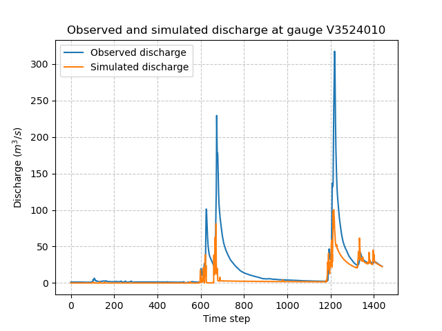
As the hydrograph shows, the simulated discharge is quite different from the observed discharge at this gauge. Obviously, we ran a forward run with the default smash rainfall-runoff parameter set. We can now try to run an optimization to minimize the misfit between the simulated and observed discharge.

Optimization

Similar to the Model.forward_run method, an optimization can be called with the Model.optimize method.

In [91]: model.optimize()

And visualize again the simulated discharge compared to the observed discharge, but this time with optimized model parameters.

In [92]: code = model.mesh.code[0]

In [93]: plt.plot(model.response_data.q[0, :], label="Observed discharge");

In [94]: plt.plot(model.response.q[0, :], label="Simulated discharge");

In [95]: plt.xlabel("Time step");

In [96]: plt.ylabel("Discharge ($m^3/s$)");

In [97]: plt.grid(ls="--", alpha=.7);

In [98]: plt.legend();

In [99]: plt.title(f"Observed and simulated discharge at gauge {code}");

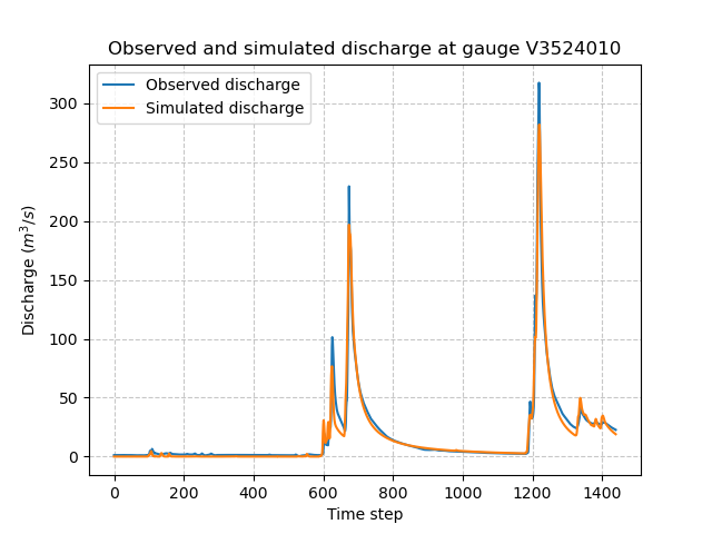
Of course, the hydrological model optimization problem is a complex one and there are many strategies that can be employed depending on the modeling goals and data available. Here, for a first tutorial, we have run a simple optimization with the function’s default parameters (SBS global optimization algorithm). The end of this section will be dedicated to a brief explanation of the information associated with the optimization performed.

First, several information were displayed on the screen during optimization

At iterate      0    nfg =     1    J =      0.695010    ddx = 0.64
At iterate      1    nfg =    30    J =      0.098411    ddx = 0.64
At iterate      2    nfg =    59    J =      0.045409    ddx = 0.32
At iterate      3    nfg =    88    J =      0.038182    ddx = 0.16
At iterate      4    nfg =   117    J =      0.037362    ddx = 0.08
At iterate      5    nfg =   150    J =      0.037087    ddx = 0.02
At iterate      6    nfg =   183    J =      0.036800    ddx = 0.02
At iterate      7    nfg =   216    J =      0.036763    ddx = 0.01
CONVERGENCE: DDX < 0.01

These lines show the different iterations of the optimization with information on the number of iterations, the number of cumulative evaluations nfg (number of foward runs performed within each iteration of the optimization algorithm), the value of the cost function to minimize J and the value of the adaptive descent step ddx of this heuristic search algorihtm. So, to summarize, the optimization algorithm has converged after 7 iterations by reaching the descent step tolerance criterion of 0.01. This optimization required to perform 216 forward run evaluations and leads to a final cost function value on the order of 0.04.

Then, we can ask which cost function J has been minimized and which parameters have been optimized. So, by default, the cost function to be minimized is one minus the Nash-Sutcliffe efficiency nse (\(1 - \text{NSE}\)) and the optimized parameters are the set of rainfall-runoff parameters (cp, ct, kexc and llr). In the current configuration spatially uniform parameters were optimized, i.e. a spatially uniform map for each parameter. We can visualize the optimized rainfall-runoff parameters.

In [100]: ind = tuple(model.mesh.gauge_pos[0, :])

In [101]: opt_parameters = {
   .....:     k: model.get_rr_parameters(k)[ind] for k in ["cp", "ct", "kexc", "llr"]
   .....: } # A dictionary comprehension
   .....: 

In [102]: opt_parameters
Out[102]: 
{'cp': np.float32(75.816666),
 'ct': np.float32(255.8543),
 'kexc': np.float32(-1.3692871),
 'llr': np.float32(30.552221)}

Save Model

Before finishing this first tutorial, like the setup and mesh dictionaries, the smash.Model object, including the optimized parameters, can be saved to HDF5 format and read back using the smash.io.save_model and smash.io.read_model functions, respectively.

In [103]: smash.io.save_model(model, "model.hdf5")

In [104]: model = smash.io.read_model("model.hdf5")

In [105]: model
Out[105]: 
Model
    atmos_data: ['mean_pet', 'mean_prcp', '...', 'sparse_prcp', 'sparse_snow']
    mesh: ['active_cell', 'area', '...', 'xres', 'ymax']
    physio_data: ['descriptor', 'l_descriptor', 'u_descriptor']
    response: ['q']
    response_data: ['q']
    rr_final_states: ['keys', 'values']
    rr_initial_states: ['keys', 'values']
    rr_parameters: ['keys', 'values']
    serr_mu_parameters: ['keys', 'values']
    serr_sigma_parameters: ['keys', 'values']
    setup: ['adjust_interception', 'compute_mean_atmos', '...', 'temp_access', 'temp_directory']
    u_response_data: ['q_stdev']

This concludes this first tutorial on smash. The next quickstart tutorial will cover all of mainland France.