Lez - Split Sample Test

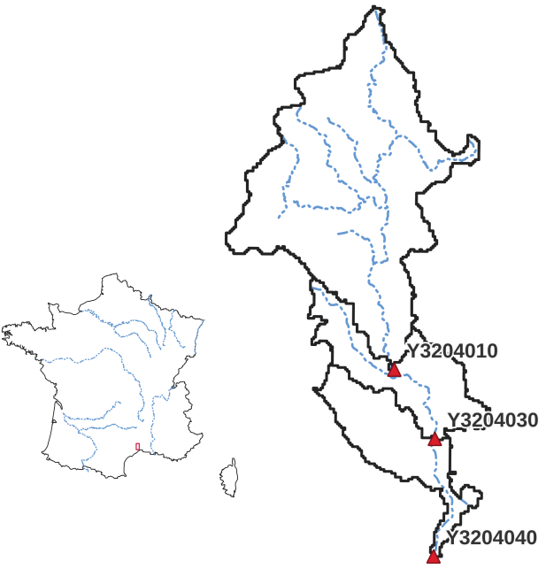
This third and last quickstart tutorial on smash will be carried out on another French catchment, the Lez at Lattes. The objective is to set up an optimization with split sample test [Klemeš, 1986], i.e. cross-calibration and temporal validation over two distinct periods p1 and p2.

Required data

You need first to download all the required data.

Download

If the download was successful, a file named Lez-dataset.tar should be available. We can switch to the directory where this file has been downloaded and extract it using the following command:

tar xf Lez-dataset.tar

Now a folder called Lez-dataset should be accessible and contain the following files and folders:

• France_flwdir.tif

  A GeoTiff file containing the flow direction data,

• gauge_attributes.csv

  A csv file containing the gauge attributes (gauge coordinates, drained area and code),

• prcp

  A directory containing precipitation data in GeoTiff format with the following directory structure: %Y/%m (2012/08),

• pet

  A directory containing daily interannual potential evapotranspiration data in GeoTiff format,

• qobs

  A directory containing the observed discharge data in csv format,

• descriptor

  A directory containing physiographic descriptors in GeoTiff format.

We can open a Python interface. The current working directory will be assumed to be the directory where the Lez-dataset is located.

Open a Python interface:

python3

Imports

We will first import everything we need in this tutorial.

In [1]: import smash

In [2]: import numpy as np

In [3]: import pandas as pd

In [4]: import matplotlib.pyplot as plt

Model creation

Model setup creation

Since we are going to work on two different periods, each of 6 months, we need to create two setups dictionaries where the only difference will be in the simulation period arguments start_time and end_time. The first period p1 will run from 2012-08-01 to 2013-01-31 and the second, from 2013-02-01 to 2013-07-31.

In [5]: setup_p1 = {
   ...:     "start_time": "2012-08-01",
   ...:     "end_time": "2013-01-31",
   ...:     "dt": 86_400, # daily time step
   ...:     "hydrological_module": "gr4",
   ...:     "routing_module": "lr",
   ...:     "read_prcp": True,
   ...:     "prcp_directory": "./Lez-dataset/prcp",
   ...:     "read_pet": True,
   ...:     "pet_directory": "./Lez-dataset/pet",
   ...:     "read_qobs": True,
   ...:     "qobs_directory": "./Lez-dataset/qobs"
   ...: }
   ...: 

In [6]: setup_p2 = {
   ...:     "start_time": "2013-02-01",
   ...:     "end_time": "2013-07-31",
   ...:     "dt": 86_400, # daily time step
   ...:     "hydrological_module": "gr4",
   ...:     "routing_module": "lr",
   ...:     "read_prcp": True,
   ...:     "prcp_directory": "./Lez-dataset/prcp",
   ...:     "read_pet": True,
   ...:     "pet_directory": "./Lez-dataset/pet",
   ...:     "read_qobs": True,
   ...:     "qobs_directory": "./Lez-dataset/qobs"
   ...: }
   ...: 

Model mesh creation

For the mesh, there is no need to generate two different meshes dictionaries, the same one can be used for both time periods. Similar to the Cance tutorial, we are going to create a mesh from the attributes of the catchment gauges.

In [7]: gauge_attributes = pd.read_csv("./Lez-dataset/gauge_attributes.csv")

In [8]: mesh = smash.factory.generate_mesh(
   ...:     flwdir_path="./Lez-dataset/France_flwdir.tif",
   ...:     x=list(gauge_attributes["x"]),
   ...:     y=list(gauge_attributes["y"]),
   ...:     area=list(gauge_attributes["area"] * 1e6), # Convert km² to m²
   ...:     code=list(gauge_attributes["code"]),
   ...: )
   ...: 

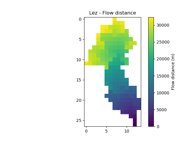
And quickly verify that the generated mesh is correct

In [9]: plt.imshow(mesh["flwdst"]);

In [10]: plt.colorbar(label="Flow distance (m)");

In [11]: plt.title("Lez - Flow distance");

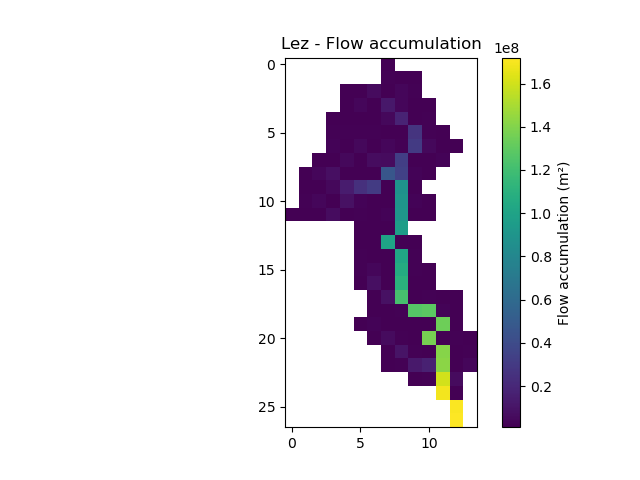
In [12]: plt.imshow(mesh["flwacc"]);

In [13]: plt.colorbar(label="Flow accumulation (m²)");

In [14]: plt.title("Lez - Flow accumulation");

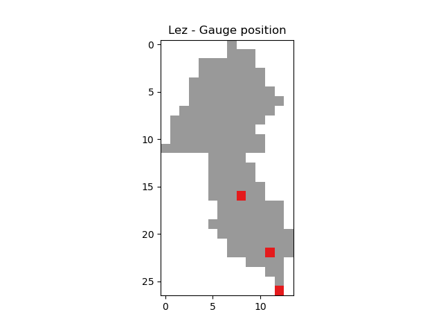
In [15]: base = np.zeros(shape=(mesh["nrow"], mesh["ncol"]))

In [16]: base = np.where(mesh["active_cell"] == 0, np.nan, base)

In [17]: for pos in mesh["gauge_pos"]:
   ....:     base[pos[0], pos[1]] = 1
   ....: 

In [18]: plt.imshow(base, cmap="Set1_r");

In [19]: plt.title("Lez - Gauge position");

Then, we can initialize the two smash.Model objects

In [20]: model_p1 = smash.Model(setup_p1, mesh)
</> Computing mean atmospheric data

In [21]: model_p2 = smash.Model(setup_p2, mesh)
</> Computing mean atmospheric data

Model simulation

Optimization

First, we will optimize both models for each period to generate two sets of optimized rainfall-runoff parameters. So far, to optimize, we have called the method associated with the smash.Model object Model.optimize. This method will modify the associated object in place (i.e. the values of the rainfall-runoff parameters after calling this function are modified). Here, we want to optimize the model but still keep this model object to run the validation afterwards. To do this, instead of calling the Model.optimize method, we can call the smash.optimize function, which is identical but takes a smash.Model object as input and returns a copy of it. This method allows you to optimize a smash.Model object and store the results in another object without modifying the initial one.

Similar to the Cance tutorial, we will perform a simple spatially uniform optimization (SBS global optimization algorithm) of the rainfall-runoff parameters by minimizing the cost function equal to one minus the Nash-Sutcliffe efficiency on the most downstream gauge.

In [22]: model_p1_opt = smash.optimize(model_p1)

In [23]: model_p2_opt = smash.optimize(model_p2)

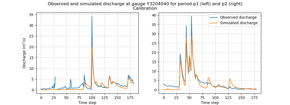
We can take a look at the hydrographs and optimized rainfall-runoff parameters.

In [24]: code = model_p1.mesh.code[0]

In [25]: f, (ax1, ax2) = plt.subplots(1, 2, figsize=(11, 4));

In [26]: qobs = model_p1_opt.response_data.q[0,:].copy()

In [27]: qobs = np.where(qobs < 0, np.nan, qobs) # To deal with missing values

In [28]: qsim = model_p1_opt.response.q[0,:]

In [29]: ax1.plot(qobs);

In [30]: ax1.plot(qsim);

In [31]: ax1.grid(ls="--", alpha=.7);

In [32]: ax1.set_xlabel("Time step");

In [33]: ax1.set_ylabel("Discharge ($m^3/s$)");

In [34]: qobs = model_p2_opt.response_data.q[0,:].copy()

In [35]: qobs = np.where(qobs < 0, np.nan, qobs) # To deal with missing values

In [36]: qsim = model_p2_opt.response.q[0,:]

In [37]: ax2.plot(qobs, label="Observed discharge");

In [38]: ax2.plot(qsim, label="Simulated discharge");

In [39]: ax2.grid(ls="--", alpha=.7);

In [40]: ax2.set_xlabel("Time step");

In [41]: ax2.legend();

In [42]: f.suptitle(
   ....:     f"Observed and simulated discharge at gauge {code}"
   ....:     " for period p1 (left) and p2 (right)\nCalibration"
   ....: );
   ....: 

In [43]: ind = tuple(model_p1.mesh.gauge_pos[0, :])

In [44]: opt_parameters_p1 = {
   ....:     k: model_p1_opt.get_rr_parameters(k)[ind] for k in ["cp", "ct", "kexc", "llr"]
   ....: } # A dictionary comprehension
   ....: 

In [45]: opt_parameters_p2 = {
   ....:     k: model_p2_opt.get_rr_parameters(k)[ind] for k in ["cp", "ct", "kexc", "llr"]
   ....: } # A dictionary comprehension
   ....: 

In [46]: opt_parameters_p1
Out[46]: 
{'cp': np.float32(160.85303),
 'ct': np.float32(33.92805),
 'kexc': np.float32(-0.0010485138),
 'llr': np.float32(562.4298)}

In [47]: opt_parameters_p2
Out[47]: 
{'cp': np.float32(9.942335e-05),
 'ct': np.float32(107.30205),
 'kexc': np.float32(-2.3589046),
 'llr': np.float32(498.9533)}

Temporal validation

Rainfall-runoff parameters transfer

We can now transfer the optimized rainfall-runoff parameters for each calibration period to the respective validation period. We will transfer the rainfall-runoff parameters from model_p1_opt to model_p2 and from model_p2_opt to model_p1. There are several ways to do this:

• Transfer all rainfall-runoff parameters at once

  All rainfall-runoff parameters are stored in the variable values of the object Model.rr_parameters. We can therefore pass the whole array of rainfall-runoff parameters from one object to the other.

  In [48]: model_p1.rr_parameters.values = model_p2_opt.rr_parameters.values.copy()
  
  In [49]: model_p2.rr_parameters.values = model_p1_opt.rr_parameters.values.copy()
  

  Note

  A deep copy is recommended to avoid that the rainfall-runoff parameters between each object become shallow copies and so that the modification of one of the arrays leads to the modification of another.

• Transfer each rainfall-runoff parameter one by one

  It is also possible to loop on each rainfall-runoff parameter and assign new rainfall-runoff parameter by passing by getters and setters

  In [50]: for key in model_p1.rr_parameters.keys:
     ....:     model_p1.set_rr_parameters(key, model_p2_opt.get_rr_parameters(key))
     ....:     model_p2.set_rr_parameters(key, model_p1_opt.get_rr_parameters(key))
     ....: 
  

  Note

  This method allows, instead of looping on all rainfall-runoff parameters, to loop only on some. We can replace model_p1.rr_parameters.keys by ["cp", "ct"] for example

Forward run

Once the rainfall-runoff parameters have been transferred, we can proceed with the validation forward runs by calling the Model.forward_run method.

In [51]: model_p1.forward_run()
</> Forward Run

In [52]: model_p2.forward_run()
</> Forward Run

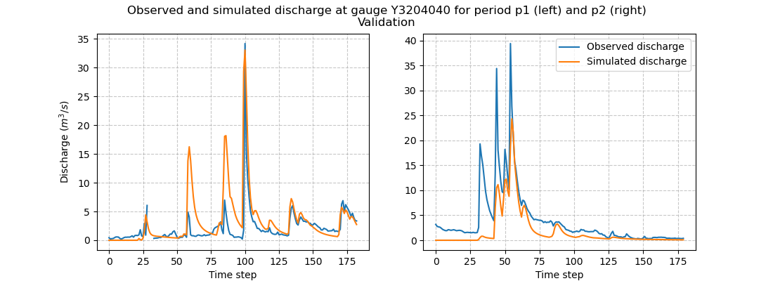
and visualize hydrographs

In [53]: code = model_p1.mesh.code[0]

In [54]: f, (ax1, ax2) = plt.subplots(1, 2, figsize=(11, 4));

In [55]: qobs = model_p1.response_data.q[0,:].copy()

In [56]: qobs = np.where(qobs < 0, np.nan, qobs) # To deal with missing values

In [57]: qsim = model_p1.response.q[0,:]

In [58]: ax1.plot(qobs);

In [59]: ax1.plot(qsim);

In [60]: ax1.grid(ls="--", alpha=.7);

In [61]: ax1.set_xlabel("Time step");

In [62]: ax1.set_ylabel("Discharge ($m^3/s$)");

In [63]: qobs = model_p2.response_data.q[0,:].copy()

In [64]: qobs = np.where(qobs < 0, np.nan, qobs) # To deal with missing values

In [65]: qsim = model_p2.response.q[0,:]

In [66]: ax2.plot(qobs, label="Observed discharge");

In [67]: ax2.plot(qsim, label="Simulated discharge");

In [68]: ax2.grid(ls="--", alpha=.7);

In [69]: ax2.set_xlabel("Time step");

In [70]: ax2.legend();

In [71]: f.suptitle(
   ....:     f"Observed and simulated discharge at gauge {code}"
   ....:     " for period p1 (left) and p2 (right)\nValidation"
   ....: );
   ....: 

Model performances

Finally, we can look at calibration and validation performances using certain metrics. Using the function smash.metrics, you can compute one metric of your choice (among those available) for all the gauges that make up the mesh. Here, we are interested in the nse (the calibration metric) and the kge for the downstream gauge only. We will create two pandas.DataFrame, one for the calibration performances and the other for the validation performances.

In [72]: metrics = ["nse", "kge"]

In [73]: perf_cal = pd.DataFrame(index=["p1", "p2"], columns=metrics)

In [74]: perf_val = perf_cal.copy()

In [75]: for m in metrics:
   ....:     perf_cal.loc["p1", m] = np.round(smash.metrics(model_p1_opt, metric=m)[0], 2)
   ....: 

In [76]: for m in metrics:
   ....:     perf_cal.loc["p2", m] = np.round(smash.metrics(model_p2_opt, metric=m)[0], 2)
   ....: 

In [77]: for m in metrics:
   ....:     perf_val.loc["p1", m] = np.round(smash.metrics(model_p1, metric=m)[0], 2)
   ....: 

In [78]: for m in metrics:
   ....:     perf_val.loc["p2", m] = np.round(smash.metrics(model_p2, metric=m)[0], 2)
   ....: 

In [79]: perf_cal # Calibration performances
Out[79]: 
     nse   kge
p1  0.65   0.7
p2  0.86  0.88

In [80]: perf_val # Validation performances
Out[80]: 
     nse   kge
p1 -0.38  0.17
p2  0.53  0.35