Automatic meshing

This section aims to go into detail on how to generate a mesh automatically.

First, open a Python interface:

python3

Imports

In [1]: import smash

In [2]: import numpy as np

In [3]: import matplotlib.pyplot as plt

Single gauge mesh

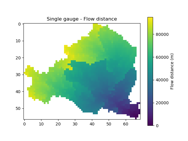
The mesh on a single gauge is applied on the catchment of L'Ardèche (TODO add fig).

The minimum data to fill in are the coordinates of the outlet and the area in m².

In [4]: (x, y) = 823_629, 6_358_543

In [5]: area = 2264 * 1e6

Then we need to provide the path to the flow directions raster file. Here we will directly load the 1km France flow directions from the smash.load_dataset() method.

Warning

The flow directions file and the (x, y) coordinates must be in the same CRS. Here we use the Lambert93 cartesien projection (EPSG:2154).

In [6]: flwdir = smash.load_dataset("flwdir")

We can now generate the mesh using the smash.generate_mesh() method.

In [7]: mesh = smash.generate_mesh(
   ...:         path=flwdir,
   ...:         x=x,
   ...:         y=y,
   ...:         area=area,
   ...: )
   ...: 

Check output

Once the mesh is generated, the user can visualize the output to confirm that the meshing has been done correctly.

The simpliest way to check if the meshing is correct (or at least, not completely wrong) is to check the modeled x, y and area compared to the observed data.

# GAUGE POS STORE (ROW, COL) INDICES
# ROW
In [8]: y_mod = mesh["ymax"] - mesh["gauge_pos"][0, 0] * mesh["dx"]

# COL
In [9]: x_mod = mesh["xmin"] + mesh["gauge_pos"][0, 1] * mesh["dx"]

In [10]: x_mod, x
Out[10]: (823000.0, 823629)

In [11]: y_mod, y
Out[11]: (6358000.0, 6358543)

In [12]: distance = np.sqrt((x - x_mod) ** 2 + (y - y_mod) ** 2)

In [13]: distance
Out[13]: 830.957279286968

The distance between the observed outlet and the modeled outlet is approximately 831 meters. Concerning the area.

In [14]: area_mod = mesh["area"][0]

In [15]: area_mod, area
Out[15]: (2257000000.0, 2264000000.0)

In [16]: rel_err = (area - area_mod) / area

In [17]: rel_err
Out[17]: 0.0030919010600706713

The relative error between observed area and modeled area is approximately 0.3%.

Then, we can visualize any map such as the flow distances.

In [18]: plt.imshow(mesh["flwdst"]);

In [19]: plt.colorbar(label="Flow distance (m)");

In [20]: plt.title("Single gauge - Flow distance");

Missmatching data

It can sometimes happen that the meshing observed data (x, y, and area) is not consistent with the flow directions. We will assume in the following case that we have a shift of the catchment outlet real coordinates.

In [21]: x_off = x + 2_000

In [22]: mesh_off = smash.generate_mesh(
   ....:         path=flwdir,
   ....:         x=x_off,
   ....:         y=y,
   ....:         area=area,
   ....: )
   ....: 

In [23]: area_mod = mesh_off["area"][0]

In [24]: area_mod, area
Out[24]: (26000000.0, 2264000000.0)

In [25]: rel_err = (area - area_mod) / area

In [26]: rel_err
Out[26]: 0.9885159010600707

In [27]: plt.imshow(mesh_off["flwdst"]);

In [28]: plt.colorbar(label="Flow distance (m)");

In [29]: plt.title("Missmatch single gauge - Flow distance");

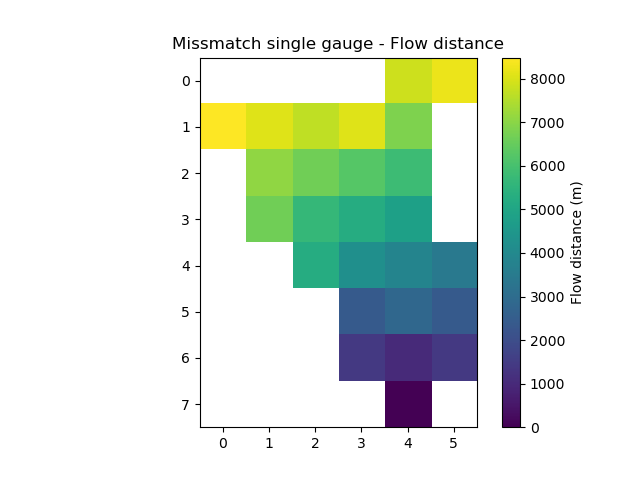
As shown by the relative error on the areas (98%) and the flow distances, we did not generate the expected meshing for the catchment.

Max depth search

One way to circumvent this type of problem is to allow the meshing algorithm to search for cells further away from the real coordinates of the outlet in order to retrieve a relative error on the coherent areas. This can be done by entering the maximum acceptable distance max_depth in the function. This value is by default set to 1, i.e. we take the cell minimizing the error between observed and modeled area for a circle of 1 around the observed outlet. Setting this value to n \(\forall n \in \mathbb{N}^*\), allows to look at a circle of n around the outlet. This argument is useful to find the catchment you want to model if there are small inconsistencies between the flow directions and the observed data. You have to be careful with this argument. If the value of max_depth is too large, it is possible that the algorithm finds a point minimizing the relative error on the areas but for a different catchment.

Let’s try a max_depth set to 2.

In [30]: mesh_off = smash.generate_mesh(
   ....:         path=flwdir,
   ....:         x=x_off,
   ....:         y=y,
   ....:         area=area,
   ....:         max_depth=2,
   ....: )
   ....: 

In [31]: area_mod = mesh_off["area"][0]

In [32]: area_mod, area
Out[32]: (2257000000.0, 2264000000.0)

In [33]: rel_err = (area - area_mod) / area

In [34]: rel_err
Out[34]: 0.0030919010600706713

In [35]: plt.imshow(mesh_off["flwdst"]);

In [36]: plt.colorbar(label="Flow distance (m)");

In [37]: plt.title("Max depth single gauge - Flow distance");

We allowed the algorithm to look for an outlet further around the real outlet and we found the initial mesh.

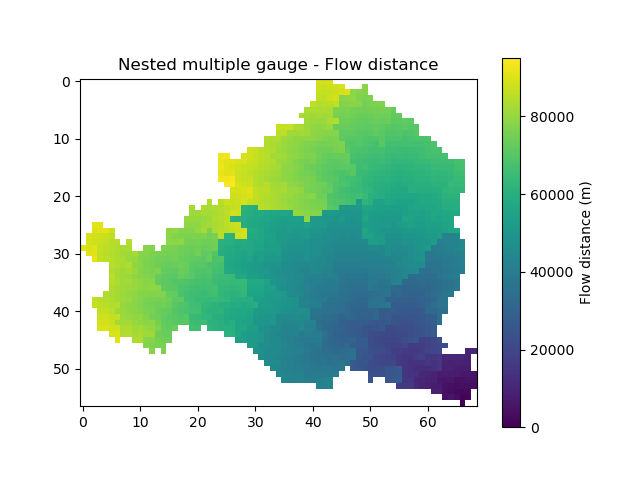
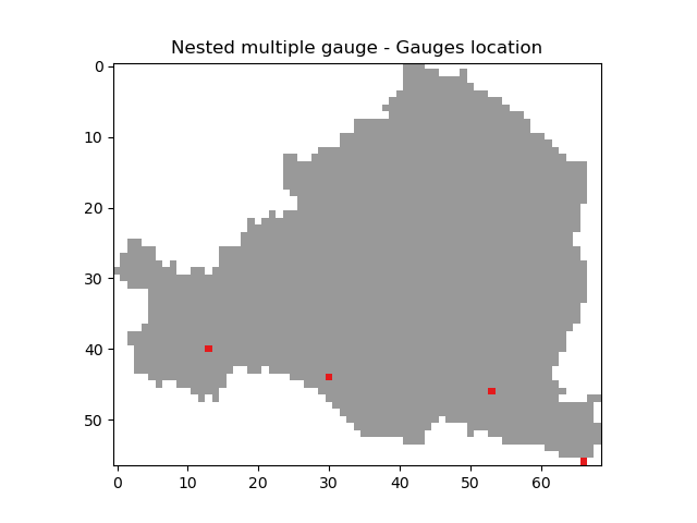
Nested multiple gauge mesh

The mesh on nested multiple gauge is still applied on the catchment of L'Ardèche for 4 gauges (TODO add fig).

Instead of being float, x, y and area are lists of float.

In [38]: x = np.array([786875, 770778, 810350, 823714])

In [39]: y = np.array([6370217, 6373832, 6367508, 6358435])

In [40]: area = np.array([496, 103, 1958, 2264]) * 1e6

Note

x, y and area are NumPy arrays but could’ve been lists, tuples or sets (any list-like object) but working with NumPy arrays makes the operations easier.

Then call the smash.generate_mesh() method.

In [41]: mesh = smash.generate_mesh(
   ....:         path=flwdir,
   ....:         x=x,
   ....:         y=y,
   ....:         area=area,
   ....: )
   ....: 

Check output

Same as the single gauge, we can confirm that the mesh has been correctly done by checking distances and areas.

In [42]: y_mod = mesh["ymax"] - mesh["gauge_pos"][:, 0] * mesh["dx"]

In [43]: x_mod = mesh["xmin"] + mesh["gauge_pos"][:, 1] * mesh["dx"]

In [44]: distance = np.sqrt((x - x_mod) ** 2 + (y - y_mod)** 2)

In [45]: rel_err = (area - mesh["area"]) / area

In [46]: distance
Out[46]: array([250.42763426, 795.93215791, 603.79135469, 836.07475742])

In [47]: rel_err
Out[47]: array([ 0.        , -0.03883495,  0.00153214,  0.0030919 ])

As well as visualize the flow distances map, which will be the same as the single gauge case because the flow distances are only calculated for the most downstream gauge in case of nested gauges.

In [48]: plt.imshow(mesh["flwdst"]);

In [49]: plt.colorbar(label="Flow distance (m)");

In [50]: plt.title("Nested multiple gauge - Flow distance");

Gauges location

One way to visualize where the 4 gauges are located.

In [51]: canvas = np.zeros(shape=mesh["flwdir"].shape)

In [52]: canvas = np.where(mesh["active_cell"] == 0, np.nan, canvas)

In [53]: for pos in mesh["gauge_pos"]:
   ....:     canvas[tuple(pos)] = 1
   ....: 

In [54]: plt.imshow(canvas, cmap="Set1_r");

In [55]: plt.title("Nested multiple gauge - Gauges location");

Gauges code

When working with a single gauge, it is not usefull to give a code for the gauge. When working with multiple gauge, especially in case of optimization, we need to know how to call the gauges. By default, if no code are given to the smash.generate_mesh() method, the codes are the following.

In [56]: mesh["code"]
Out[56]: array(['_c0', '_c1', '_c2', '_c3'], dtype='<U3')

The gauges code are always sorted in the same way than the gauges location.

The default codes are generally not enought explicit and the user can provide it’s own gauges code by directly change the mesh dictionary value or filling in the argument code in the smash.generate_mesh()

In [57]: code = np.array(["V5045030", "V5046610", "V5054010", "V5064010"])

In [58]: code
Out[58]: array(['V5045030', 'V5046610', 'V5054010', 'V5064010'], dtype='<U8')

In [59]: mesh["code"] = code.copy()

In [60]: mesh = smash.generate_mesh(
   ....:         path=flwdir,
   ....:         x=x,
   ....:         y=y,
   ....:         area=area,
   ....:         code=code,
   ....: )
   ....: 

In [61]: mesh["code"]
Out[61]: array(['V5045030', 'V5046610', 'V5054010', 'V5064010'], dtype='<U8')

Warning

When setting gauges code directly in the mesh dictionary, the value must be a NumPy array. Otherwise, similar to the arguments x, y and area, the codes can be any list-like object (NumPy array, list, tuple or set).

Non-nested multiple gauge mesh

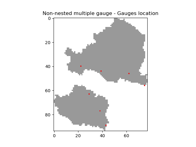
The mesh on non-nested multiple gauge is still applied on the catchment of L'Ardèche for 4 gauges and on the catchment of Le Gardon for 3 gauges (TODO add fig).

There is no difference in the way the method smash.generate_mesh() is called between nested and non-nested gauges.

So we fill in x, y and the area.

In [62]: x = np.array(
   ....:     [786875, 770778, 810350, 823714, 786351, 778264, 792628]
   ....: )
   ....: 

In [63]: y = np.array(
   ....:     [6370217, 6373832, 6367508, 6358435, 6336298, 6349858, 6324727]
   ....: )
   ....: 

In [64]: area = np.array(
   ....:     [496, 103, 1958, 2264, 315, 115, 1093]
   ....: ) * 1e6
   ....: 

Then call the smash.generate_mesh() method.

In [65]: mesh = smash.generate_mesh(
   ....:         path=flwdir,
   ....:         x=x,
   ....:         y=y,
   ....:         area=area,
   ....: )
   ....: 

In [66]: plt.imshow(mesh["flwdst"]);

In [67]: plt.colorbar(label="Flow distance (m)");

In [68]: plt.title("Non-nested multiple gauge - Flow distance");

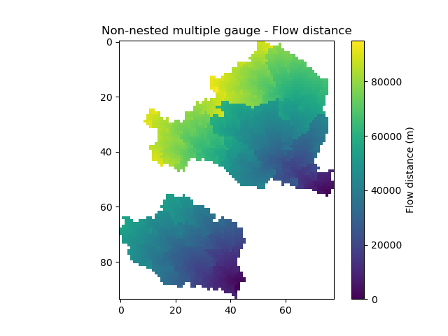
The mesh has been generated for two groups of catchments which are non-nested.

Note

The flow distances are always calculated on the most downstream gauge. In case of non-nested groups of catchments, the flow distance are calculated for each group on the most downstream gauge.

Finally, visualize the gauge positions for this mesh.

In [69]: canvas = np.zeros(shape=mesh["flwdir"].shape)

In [70]: canvas = np.where(mesh["active_cell"] == 0, np.nan, canvas)

In [71]: for pos in mesh["gauge_pos"]:
   ....:     canvas[tuple(pos)] = 1
   ....: 

In [72]: plt.imshow(canvas, cmap="Set1_r");

In [73]: plt.title("Non-nested multiple gauge - Gauges location");