Practice case#
The Practice case is an introduction to smash for new users. The objective of this section is to create the dataset to run smash from scratch and get an overview of what is available. More details are provided on a real case available in the User Guide section: Real case - Cance.
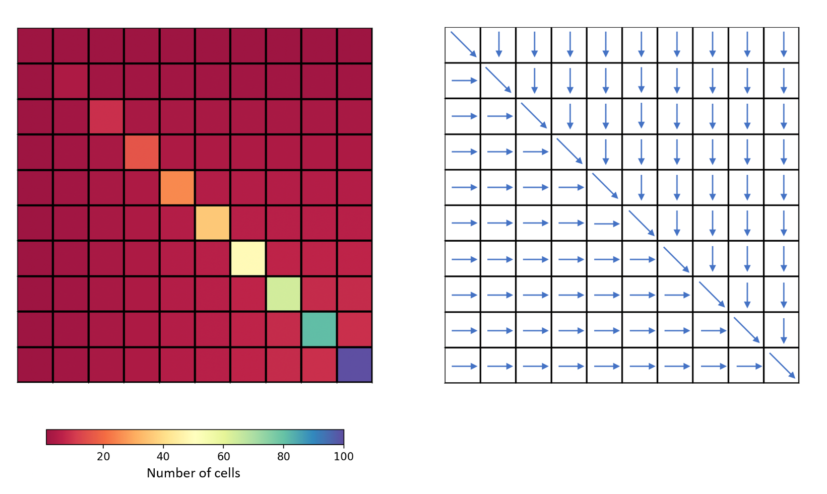
For this case, a fictitious square-shaped catchment of size 10 x 10 km² will be created with the following flow accumulation and flow directions:
First, open a Python interface:
python3
Imports#
In [1]: import smash

In [2]: import numpy as np

In [3]: import matplotlib.pyplot as plt
Warning
The wrapping of Fortran code in Python requires the use of the f90wrap package, which itself uses f2py. Thus, the NumPy package is essential in the management of arguments. A knowledge of this package is advised in the use of
smash.The Matplotlib package is the visualization package used in the
smashdocumentation but any tool can be used.
Model object creation#
Creating a Model requires two input arguments: setup and mesh.
Setup argument creation#
setup is a dictionary that allows to initialize Model (i.e. allocate the necessary Fortran arrays).
Note
Each key and associated values that can be passed into the setup dictionary are detailed in the User Guide section: Model initialization.
A minimal setup configuration is:
dt: the calculation time step in s,start_time: the beginning of the simulation,end_time: the end of the simulation.
In [4]: setup = {
   ...:     "dt": 3_600,
   ...:     "start_time": "2020-01-01 00:00",
   ...:     "end_time": "2020-01-04 00:00",
   ...: }
   ...:
Mesh argument creation#
mesh is a dictionary that allows to initialize Model (i.e. allocate the necessary Fortran arrays).
Note
Each key and associated values that can be passed into the
meshdictionary are detailed in the User Guide section: Model initialization.In the Practice case, because the catchment is ficticious, we create the
meshdictionary ourselves. In the case of a real catchment, the meshing generation can be done automatically via the meshing methodsmash.generate_mesh(). More details can be found in the User Guide section: Automatic meshing.
First part of mesh configuration is:
dx: the calculation spatial step in m,nrow: the number of rows,ncol: the number of columns,ng: the number of gauges,nac: the number of cells that contribute to any gauge discharge (here the full grid contributes),area: the catchment area in m²,gauge_pos: the gauge position in the grid (here lower right corner [9,9]),code: the gauge code.
In [5]: dx = 1_000

In [6]: (nrow, ncol) = (10, 10)

In [7]: mesh = {
   ...:     "dx": dx,
   ...:     "nrow": nrow,
   ...:     "ncol": ncol,
   ...:     "ng": 1,
   ...:     "nac": nrow * ncol,
   ...:     "area": nrow * ncol * (dx ** 2),
   ...:     "gauge_pos": np.array([9, 9], dtype=np.int32),
   ...:     "code": np.array(["Practice_case"])
   ...: }
   ...:
Second part of mesh configuration is:
flwdir: the flow directions,flwacc: the flow accumulation in number of cells.
In [8]: mesh["flwdir"] = np.array(
   ...:     [
   ...:     [4, 5, 5, 5, 5, 5, 5, 5, 5, 5],
   ...:     [3, 4, 5, 5, 5, 5, 5, 5, 5, 5],
   ...:     [3, 3, 4, 5, 5, 5, 5, 5, 5, 5],
   ...:     [3, 3, 3, 4, 5, 5, 5, 5, 5, 5],
   ...:     [3, 3, 3, 3, 4, 5, 5, 5, 5, 5],
   ...:     [3, 3, 3, 3, 3, 4, 5, 5, 5, 5],
   ...:     [3, 3, 3, 3, 3, 3, 4, 5, 5, 5],
   ...:     [3, 3, 3, 3, 3, 3, 3, 4, 5, 5],
   ...:     [3, 3, 3, 3, 3, 3, 3, 3, 4, 5],
   ...:     [3, 3, 3, 3, 3, 3, 3, 3, 3, 4],
   ...:     ],
   ...:     dtype=np.int32,
   ...: )
   ...:

In [9]: mesh["flwacc"] = np.array(
   ...:     [
   ...:            [1, 1, 1, 1, 1, 1, 1, 1, 1, 1],
   ...:            [1, 4, 2, 2, 2, 2, 2, 2, 2, 2],
   ...:            [1, 2, 9, 3, 3, 3, 3, 3, 3, 3],
   ...:            [1, 2, 3, 16, 4, 4, 4, 4, 4, 4],
   ...:            [1, 2, 3, 4, 25, 5, 5, 5, 5, 5],
   ...:            [1, 2, 3, 4, 5, 36, 6, 6, 6, 6],
   ...:            [1, 2, 3, 4, 5, 6, 49, 7, 7, 7],
   ...:            [1, 2, 3, 4, 5, 6, 7, 64, 8, 8],
   ...:            [1, 2, 3, 4, 5, 6, 7, 8, 81, 9],
   ...:            [1, 2, 3, 4, 5, 6, 7, 8, 9, 100],
   ...:         ],
   ...:         dtype=np.int32,
   ...:     )
   ...:
Finally, the calculation path (path) must be provided (ascending order of flow accumulation). This can be directly computed from flwacc and numpy methods.
In [10]: ind_path = np.unravel_index(np.argsort(mesh["flwacc"], axis=None),
   ....:      mesh["flwacc"].shape)
   ....:

In [11]: mesh["path"] = np.zeros(shape=(2, mesh["flwacc"].size),
   ....:     dtype=np.int32)
   ....:

In [12]: mesh["path"][0, :] = ind_path[0]

In [13]: mesh["path"][1, :] = ind_path[1]
Once setup and mesh are filled in, a Model object can be created:
In [14]: model = smash.Model(setup, mesh)

In [15]: model
Out[15]:
Structure: 'gr-a'
Spatio-Temporal dimension: (x: 10, y: 10, time: 72)
Last update: Initialization
Note
The representation of the Model object is very simple and only displays the structure used, the dimensions and the last action that updated the object. More information on what the object contains is available below.
Viewing Model#
Once the Model object is created, it is possible to visualize what it contains through 6 attributes. This 6 attributes are Python classes that are derived from the wrapping of Fortran derived types.
Note
See details in the API Reference for the attributes:
Setup#
The Model.setup attribute contains a set of arguments necessary to initialize the Model. We have in the Setup argument creation part given values for the arguments dt, start_time and end_time. These values can be retrieved in the following way:
In [16]: model.setup.dt, model.setup.start_time, model.setup.end_time
Out[16]: (3600.0, '2020-01-01 00:00', '2020-01-04 00:00')
The other Model.setup arguments can also be viewed even if they have not been directly defined in the Model initialization. These arguments have default values in the code:
In [17]: model.setup.structure
Out[17]: 'gr-a'
If you are using IPython, tab completion allows you to visualize all the attributes and methods:
In [18]: model.setup.<TAB>
   ....: model.setup.copy(                   model.setup.prcp_directory
   ....: model.setup.daily_interannual_pet   model.setup.prcp_format
   ....: model.setup.descriptor_directory    model.setup.qobs_directory
   ....: model.setup.descriptor_format       model.setup.read_descriptor
   ....: model.setup.descriptor_name         model.setup.read_pet
   ....: model.setup.dt                      model.setup.read_prcp
   ....: model.setup.end_time                model.setup.read_qobs
   ....: model.setup.from_handle(            model.setup.save_net_prcp_domain
   ....: model.setup.mean_forcing            model.setup.save_qsim_domain
   ....: model.setup.pet_conversion_factor   model.setup.sparse_storage
   ....: model.setup.pet_directory           model.setup.start_time
   ....: model.setup.pet_format              model.setup.structure
   ....: model.setup.prcp_conversion_factor
   ....:
Mesh#
The Model.mesh attribute contains a set of arguments necessary to initialize the Model. In the Mesh argument creation part, we have given values for multiple arguments. These values can be retrieved in the following way:
In [19]: model.mesh.dx, model.mesh.nrow, model.mesh.ncol
Out[19]: (1000.0, 10, 10)
numpy array can also be viewed:
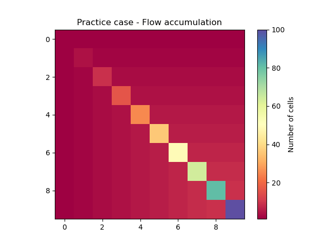
In [20]: model.mesh.flwacc
Out[20]:
array([[  1,   1,   1,   1,   1,   1,   1,   1,   1,   1],
       [  1,   4,   2,   2,   2,   2,   2,   2,   2,   2],
       [  1,   2,   9,   3,   3,   3,   3,   3,   3,   3],
       [  1,   2,   3,  16,   4,   4,   4,   4,   4,   4],
       [  1,   2,   3,   4,  25,   5,   5,   5,   5,   5],
       [  1,   2,   3,   4,   5,  36,   6,   6,   6,   6],
       [  1,   2,   3,   4,   5,   6,  49,   7,   7,   7],
       [  1,   2,   3,   4,   5,   6,   7,  64,   8,   8],
       [  1,   2,   3,   4,   5,   6,   7,   8,  81,   9],
       [  1,   2,   3,   4,   5,   6,   7,   8,   9, 100]], dtype=int32)
Or plotted using Matplotlib.
In [21]: plt.imshow(model.mesh.flwacc, cmap="Spectral");

In [22]: plt.colorbar(label="Number of cells");

In [23]: plt.title("Practice case - Flow accumulation");
If you are using IPython, tab completion allows you to visualize all the attributes and methods:
In [24]: model.mesh.<TAB>
   ....: model.mesh.active_cell   model.mesh.gauge_pos
   ....: model.mesh.area          model.mesh.nac
   ....: model.mesh.code          model.mesh.ncol
   ....: model.mesh.copy(         model.mesh.ng
   ....: model.mesh.dx            model.mesh.nrow
   ....: model.mesh.flwacc        model.mesh.path
   ....: model.mesh.flwdir        model.mesh.xmin
   ....: model.mesh.flwdst        model.mesh.ymax
   ....: model.mesh.from_handle(
   ....:
Input Data#
The Model.input_data attribute contains a set of arguments storing Model input data (i.e. atmospheric forcings, observed discharge …). As we did not specify in the Setup argument creation part a reading of input data, all tables are empty but allocated according to the size of the grid and the simulation period.
For example, the observed discharge is a numpy array of shape (1, 72). There is 1 gauge in the grid and the simulation period is up to 72 time steps. The value -99 indicates no data.
In [25]: model.input_data.qobs
Out[25]:
array([[-99., -99., -99., -99., -99., -99., -99., -99., -99., -99., -99.,
        -99., -99., -99., -99., -99., -99., -99., -99., -99., -99., -99.,
        -99., -99., -99., -99., -99., -99., -99., -99., -99., -99., -99.,
        -99., -99., -99., -99., -99., -99., -99., -99., -99., -99., -99.,
        -99., -99., -99., -99., -99., -99., -99., -99., -99., -99., -99.,
        -99., -99., -99., -99., -99., -99., -99., -99., -99., -99., -99.,
        -99., -99., -99., -99., -99., -99.]], dtype=float32)

In [26]: model.input_data.qobs.shape
Out[26]: (1, 72)
Precipitation is also a numpy array but of shape (10, 10, 72). The number of rows and columns is 10 and same as the observed dicharge, the simulation period is up to 72 time steps.
In [27]: model.input_data.prcp.shape
Out[27]: (10, 10, 72)
If you are using IPython, tab completion allows you to visualize all the attributes and methods:
In [28]: model.input_data.<TAB>
   ....: model.input_data.copy(         model.input_data.pet
   ....: model.input_data.descriptor    model.input_data.prcp
   ....: model.input_data.from_handle(  model.input_data.qobs
   ....: model.input_data.mean_pet      model.input_data.sparse_pet
   ....: model.input_data.mean_prcp     model.input_data.sparse_prcp
   ....:
Warning
It can happen, depending on the Model initialization, that some arguments of type numpy array are not accessible (unallocated array in the Fortran code). For example, we did not ask in the setup to store catchment descriptors. Access to this variable is therefore impossible and the code will return the following error:
In [29]: model.input_data.descriptor
---------------------------------------------------------------------------
ValueError                                Traceback (most recent call last)
Cell In[29], line 1
----> 1 model.input_data.descriptor

File ~/anaconda3/envs/smash-dev/lib/python3.11/site-packages/smash/solver/_mwd_input_data.py:193, in Input_DataDT.descriptor(self)
    191     descriptor = self._arrays[array_handle]
    192 else:
--> 193     descriptor = f90wrap.runtime.get_array(f90wrap.runtime.sizeof_fortran_t,
    194                             self._handle,
    195                             _solver.f90wrap_input_datadt__array__descriptor)
    196     self._arrays[array_handle] = descriptor
    197 return descriptor

ValueError: array is NULL
Parameters and States#
The Model.parameters and Model.states attributes contain a set of arguments storing Model parameters and states. This attributes contain only numpy arrays of shape (10, 10) (i.e. number of rows and columns in the grid).
In [30]: model.parameters.cp.shape, model.states.hp.shape
Out[30]: ((10, 10), (10, 10))
This arrays are filled in with uniform default values.
In [31]: model.parameters.cp, model.states.hp
Out[31]:
(array([[200., 200., 200., 200., 200., 200., 200., 200., 200., 200.],
        [200., 200., 200., 200., 200., 200., 200., 200., 200., 200.],
        [200., 200., 200., 200., 200., 200., 200., 200., 200., 200.],
        [200., 200., 200., 200., 200., 200., 200., 200., 200., 200.],
        [200., 200., 200., 200., 200., 200., 200., 200., 200., 200.],
        [200., 200., 200., 200., 200., 200., 200., 200., 200., 200.],
        [200., 200., 200., 200., 200., 200., 200., 200., 200., 200.],
        [200., 200., 200., 200., 200., 200., 200., 200., 200., 200.],
        [200., 200., 200., 200., 200., 200., 200., 200., 200., 200.],
        [200., 200., 200., 200., 200., 200., 200., 200., 200., 200.]],
       dtype=float32),
 array([[0.01, 0.01, 0.01, 0.01, 0.01, 0.01, 0.01, 0.01, 0.01, 0.01],
        [0.01, 0.01, 0.01, 0.01, 0.01, 0.01, 0.01, 0.01, 0.01, 0.01],
        [0.01, 0.01, 0.01, 0.01, 0.01, 0.01, 0.01, 0.01, 0.01, 0.01],
        [0.01, 0.01, 0.01, 0.01, 0.01, 0.01, 0.01, 0.01, 0.01, 0.01],
        [0.01, 0.01, 0.01, 0.01, 0.01, 0.01, 0.01, 0.01, 0.01, 0.01],
        [0.01, 0.01, 0.01, 0.01, 0.01, 0.01, 0.01, 0.01, 0.01, 0.01],
        [0.01, 0.01, 0.01, 0.01, 0.01, 0.01, 0.01, 0.01, 0.01, 0.01],
        [0.01, 0.01, 0.01, 0.01, 0.01, 0.01, 0.01, 0.01, 0.01, 0.01],
        [0.01, 0.01, 0.01, 0.01, 0.01, 0.01, 0.01, 0.01, 0.01, 0.01],
        [0.01, 0.01, 0.01, 0.01, 0.01, 0.01, 0.01, 0.01, 0.01, 0.01]],
       dtype=float32))
Note
The Model.states attribute stores the initial states \(h(x,0)\).
If you are using IPython, tab completion allows you to visualize all the attributes and methods:
In [32]: model.parameters.<TAB>
   ....: model.parameters.alpha         model.parameters.cusl1
   ....: model.parameters.b             model.parameters.cusl2
   ....: model.parameters.beta          model.parameters.ds
   ....: model.parameters.cft           model.parameters.dsm
   ....: model.parameters.ci            model.parameters.exc
   ....: model.parameters.clsl          model.parameters.from_handle(
   ....: model.parameters.copy(         model.parameters.ks
   ....: model.parameters.cp            model.parameters.lr
   ....: model.parameters.cst           model.parameters.ws
   ....:
In [33]: model.states.<TAB>
   ....: model.states.copy(         model.states.hlsl
   ....: model.states.from_handle(  model.states.hp
   ....: model.states.hft           model.states.hst
   ....: model.states.hi            model.states.husl1
   ....: model.states.hlr           model.states.husl2
   ....:
Output#
The last attribute, Model.output, contains a set of arguments storing Model outputs (i.e. simulated discharge, final states, cost …). The attribute values are empty as long as no simulation has been run.
If you are using IPython, tab completion allows you to visualize all the attributes and methods:
In [34]: model.output.<TAB>
   ....: model.output.copy(                   model.output.qsim
   ....: model.output.cost                    model.output.qsim_domain
   ....: model.output.from_handle(            model.output.sparse_net_prcp_domain
   ....: model.output.fstates                 model.output.sparse_qsim_domain
   ....: model.output.net_prcp_domain
   ....:
Input Data filling#
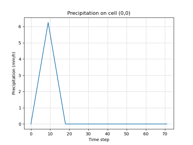
To run a simulation, the Model needs at least one precipitation and potential evapotranspiration (PET) chronicle. In this Practice case, we will impose a triangular precipitation over the simulation period, uniform on the domain and a zero PET.
In [35]: prcp = np.zeros(shape=model.input_data.prcp.shape[2], dtype=np.float32)

In [36]: tri = np.linspace(0, 6.25, 10)

In [37]: prcp[0:10] = tri

In [38]: prcp[9:19] = np.flip(tri)

In [39]: model.input_data.prcp = np.broadcast_to(
   ....:     prcp,
   ....:     model.input_data.prcp.shape,
   ....: )
   ....:

In [40]: model.input_data.pet = 0.
Checking on any cell the precipitation values:
In [41]: plt.plot(model.input_data.prcp[0,0,:]);

In [42]: plt.grid(alpha=.7, ls="--");

In [43]: plt.xlabel("Time step");

In [44]: plt.ylabel("Precipitation $(mm/h)$");

In [45]: plt.title("Precipitation on cell (0,0)");
Run#
Forward run#
The Model is finally ready to be run using the Model.run() method:
In [46]: model.run(inplace=True);

In [47]: model
Out[47]:
Structure: 'gr-a'
Spatio-Temporal dimension: (x: 10, y: 10, time: 72)
Last update: Forward Run
Once the run is done, it is possible to access the simulated discharge on the gauge via the Model.output and to plot a hydrograph.
In [48]: plt.plot(model.output.qsim[0,:]);

In [49]: plt.grid(alpha=.7, ls="--");

In [50]: plt.xlabel("Time step");

In [51]: plt.ylabel("Simulated discharge $(m^3/s)$");

In [52]: plt.title(model.mesh.code[0]);
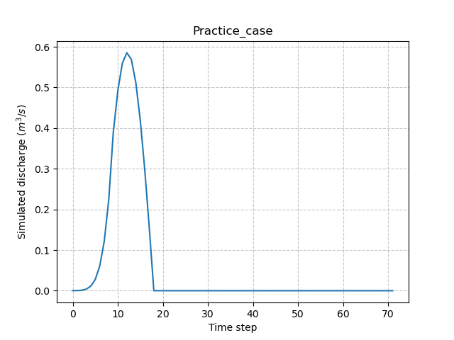
This hydrograph is the result of a forward run of the code with the default structure, parameters and initial states.
Optimization#
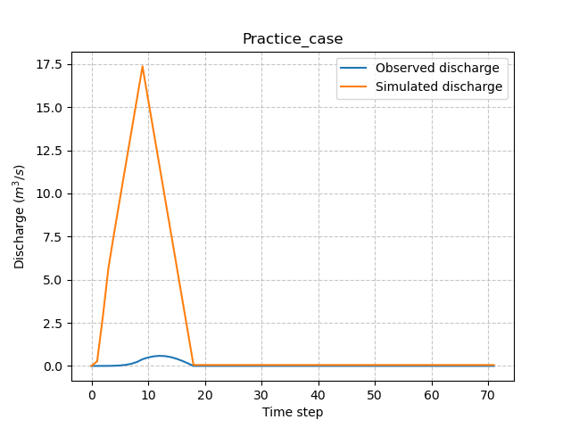
To perform an optimization, observed discharge must be provided to Model. Since the Practice case is a ficticious catchment, we will use the simulated data from the previous forward run as observed discharge.
In [53]: model.input_data.qobs = model.output.qsim.copy()
Next, we will perturb the production parameter \(\mathrm{cp}\) to generate a different hydrograph from the previous one.
In [54]: model.parameters.cp = 1
Run again to see the differences between the hydrographs.
In [55]: model.run(inplace=True);

In [56]: plt.plot(model.input_data.qobs[0,:], label="Observed discharge");

In [57]: plt.plot(model.output.qsim[0,:], label="Simulated discharge");

In [58]: plt.grid(alpha=.7, ls="--");

In [59]: plt.xlabel("Time step");

In [60]: plt.ylabel("Discharge $(m^3/s)$");

In [61]: plt.legend();

In [62]: plt.title(model.mesh.code[0]);
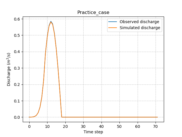
Finally, perform a spatially uniform calibration (which is default optimization) of the parameter \(\mathrm{cp}\) with the Model.optimize() method:
In [63]: model.optimize(control_vector="cp", inplace=True);

In [64]: model.parameters.cp
Out[64]:
array([[200.72115, 200.72115, 200.72115, 200.72115, 200.72115, 200.72115,
        200.72115, 200.72115, 200.72115, 200.72115],
       [200.72115, 200.72115, 200.72115, 200.72115, 200.72115, 200.72115,
        200.72115, 200.72115, 200.72115, 200.72115],
       [200.72115, 200.72115, 200.72115, 200.72115, 200.72115, 200.72115,
        200.72115, 200.72115, 200.72115, 200.72115],
       [200.72115, 200.72115, 200.72115, 200.72115, 200.72115, 200.72115,
        200.72115, 200.72115, 200.72115, 200.72115],
       [200.72115, 200.72115, 200.72115, 200.72115, 200.72115, 200.72115,
        200.72115, 200.72115, 200.72115, 200.72115],
       [200.72115, 200.72115, 200.72115, 200.72115, 200.72115, 200.72115,
        200.72115, 200.72115, 200.72115, 200.72115],
       [200.72115, 200.72115, 200.72115, 200.72115, 200.72115, 200.72115,
        200.72115, 200.72115, 200.72115, 200.72115],
       [200.72115, 200.72115, 200.72115, 200.72115, 200.72115, 200.72115,
        200.72115, 200.72115, 200.72115, 200.72115],
       [200.72115, 200.72115, 200.72115, 200.72115, 200.72115, 200.72115,
        200.72115, 200.72115, 200.72115, 200.72115],
       [200.72115, 200.72115, 200.72115, 200.72115, 200.72115, 200.72115,
        200.72115, 200.72115, 200.72115, 200.72115]], dtype=float32)

In [65]: model
Out[65]:
Structure: 'gr-a'
Spatio-Temporal dimension: (x: 10, y: 10, time: 72)
Last update: SBS Optimization
In [66]: plt.plot(model.input_data.qobs[0,:], label="Observed discharge");

In [67]: plt.plot(model.output.qsim[0,:], label="Simulated discharge");

In [68]: plt.grid(alpha=.7, ls="--");

In [69]: plt.xlabel("Time step");

In [70]: plt.ylabel("Discharge $(m^3/s)$");

In [71]: plt.legend();

In [72]: plt.title(model.mesh.code[0]);
Note
In the Practice case, we will not go into the details of the optimization which is an essential part of the smash calculation code. To go further, details can be found for the use of the Model.optimize() method in the User Guide section: TODO ref to in_depth.optimize.
Getting data#
The last step is to save what we have entered in Model (i.e. setup and mesh dictionaries) and the Model itself.
Setup argument in/out#
The setup dictionary setup, which was created in the section Setup argument creation, can be saved in YAML format via the method smash.save_setup().
In [73]: smash.save_setup(setup, "setup.yaml")
A file named setup.yaml has been created in the current working directory containing the setup dictionary information. This file can itself be opened in order to recover our initial setup dictionary via the method smash.read_setup().
In [74]: setup2 = smash.read_setup("setup.yaml")

In [75]: setup2
Out[75]: {'dt': 3600, 'end_time': '2020-01-04 00:00', 'start_time': '2020-01-01 00:00'}
Mesh argument in/out#
In a similar way to setup dictionary, the mesh dictionary created in the section Mesh argument creation can be saved to file via the method smash.save_mesh(). However, 3D numpy arrays cannot be saved in YAML format, so the mesh is saved in HDF5 format.
In [76]: smash.save_mesh(mesh, "mesh.hdf5")
A file named mesh.hdf5 has been created in the current working directory containing the mesh dictionary information. This file can itself be opened in order to recover our initial mesh dictionary via the method smash.read_mesh().
In [77]: mesh2 = smash.read_mesh("mesh.hdf5")

In [78]: mesh2
Out[78]:
{'area': 100000000,
 'dx': 1000,
 'nac': 100,
 'ncol': 10,
 'ng': 1,
 'nrow': 10,
 'code': array(['Practice_case'], dtype='<U13'),
 'flwacc': array([[  1,   1,   1,   1,   1,   1,   1,   1,   1,   1],
        [  1,   4,   2,   2,   2,   2,   2,   2,   2,   2],
        [  1,   2,   9,   3,   3,   3,   3,   3,   3,   3],
        [  1,   2,   3,  16,   4,   4,   4,   4,   4,   4],
        [  1,   2,   3,   4,  25,   5,   5,   5,   5,   5],
        [  1,   2,   3,   4,   5,  36,   6,   6,   6,   6],
        [  1,   2,   3,   4,   5,   6,  49,   7,   7,   7],
        [  1,   2,   3,   4,   5,   6,   7,  64,   8,   8],
        [  1,   2,   3,   4,   5,   6,   7,   8,  81,   9],
        [  1,   2,   3,   4,   5,   6,   7,   8,   9, 100]], dtype=int32),
 'flwdir': array([[4, 5, 5, 5, 5, 5, 5, 5, 5, 5],
        [3, 4, 5, 5, 5, 5, 5, 5, 5, 5],
        [3, 3, 4, 5, 5, 5, 5, 5, 5, 5],
        [3, 3, 3, 4, 5, 5, 5, 5, 5, 5],
        [3, 3, 3, 3, 4, 5, 5, 5, 5, 5],
        [3, 3, 3, 3, 3, 4, 5, 5, 5, 5],
        [3, 3, 3, 3, 3, 3, 4, 5, 5, 5],
        [3, 3, 3, 3, 3, 3, 3, 4, 5, 5],
        [3, 3, 3, 3, 3, 3, 3, 3, 4, 5],
        [3, 3, 3, 3, 3, 3, 3, 3, 3, 4]], dtype=int32),
 'gauge_pos': array([9, 9], dtype=int32),
 'path': array([[0, 6, 8, 5, 9, 4, 3, 2, 1, 7, 0, 0, 0, 0, 0, 0, 0, 0, 0, 1, 9, 1,
         1, 3, 1, 1, 8, 5, 4, 7, 1, 6, 2, 1, 1, 5, 8, 9, 6, 4, 7, 3, 2, 2,
         2, 2, 2, 2, 2, 3, 1, 7, 3, 5, 9, 8, 3, 3, 3, 4, 6, 3, 7, 8, 9, 4,
         4, 4, 4, 6, 5, 4, 8, 6, 7, 9, 5, 5, 5, 5, 7, 9, 6, 6, 6, 8, 7, 7,
         8, 9, 9, 2, 8, 3, 4, 5, 6, 7, 8, 9],
        [0, 0, 0, 0, 0, 0, 0, 0, 0, 0, 8, 9, 4, 3, 6, 2, 1, 7, 5, 9, 1, 2,
         3, 1, 4, 8, 1, 1, 1, 1, 6, 1, 1, 7, 5, 2, 2, 2, 2, 2, 2, 2, 3, 4,
         5, 6, 7, 9, 8, 8, 1, 3, 9, 3, 3, 3, 4, 5, 6, 3, 3, 7, 4, 4, 4, 9,
         6, 7, 8, 4, 4, 5, 5, 5, 5, 5, 7, 8, 9, 6, 6, 6, 9, 8, 7, 6, 8, 9,
         7, 7, 8, 2, 9, 3, 4, 5, 6, 7, 8, 9]], dtype=int32)}
A new Model object can be created from the read files (same as the first one).
In [79]: model2 = smash.Model(setup2, mesh2)

In [80]: model2
Out[80]:
Structure: 'gr-a'
Spatio-Temporal dimension: (x: 10, y: 10, time: 72)
Last update: Initialization
Model in/out#
The Model object can also be saved to file. Like the mesh, it will be saved in HDF5 format using the smash.save_model() method. Here, we will save the Model object model after optimization.
In [81]: smash.save_model(model, "model.hdf5")
A file named model.hdf5 has been created in the current working directory containing the model object information. This file can itself be opened in order to recover our initial model object via the method smash.read_model().
In [82]: model3 = smash.read_model("model.hdf5")

In [83]: model3
Out[83]:
Structure: 'gr-a'
Spatio-Temporal dimension: (x: 10, y: 10, time: 72)
Last update: SBS Optimization
model3 is directly the Model object itself on which the methods associated with the object are applicable.
In [84]: model3.run(inplace=True);

In [85]: model3
Out[85]:
Structure: 'gr-a'
Spatio-Temporal dimension: (x: 10, y: 10, time: 72)
Last update: Forward Run