Real case - France

A real case on the entire France is considered.

First, open a Python interface:

python3

Imports

In [1]: import smash

In [2]: import numpy as np

In [3]: import matplotlib.pyplot as plt

In [4]: from matplotlib.colors import LogNorm, SymLogNorm

Model object creation

Creating a Model requires two input arguments: setup and mesh. For this case, it is possible to directly load the both input dictionnaries using the smash.load_dataset() method.

In [5]: setup, mesh = smash.load_dataset("France")

Note

The Real case - France is very similar to the Real case - Cance except that here we do not consider catchments but a domain to make a simulation.

Setup argument

Compared to the Real case - Cance, less options have been filled in the setup dictionary.

In [6]: setup
Out[6]: 
{'structure': 'gr-a',
 'dt': 3600,
 'start_time': '2012-01-01 00:00',
 'end_time': '2012-01-02 08:00',
 'read_prcp': True,
 'prcp_format': 'tif',
 'prcp_conversion_factor': 0.1,
 'prcp_directory': '/home/fcolleoni/anaconda3/envs/smash-dev/lib/python3.11/site-packages/smash/dataset/France/prcp',
 'read_pet': True,
 'pet_format': 'tif',
 'pet_conversion_factor': 1,
 'daily_interannual_pet': True,
 'pet_directory': '/home/fcolleoni/anaconda3/envs/smash-dev/lib/python3.11/site-packages/smash/dataset/France/pet',
 'save_qsim_domain': True,
 'qobs_directory': '/home/fcolleoni/anaconda3/envs/smash-dev/lib/python3.11/site-packages/smash/dataset/France/qobs',
 'descriptor_directory': '/home/fcolleoni/anaconda3/envs/smash-dev/lib/python3.11/site-packages/smash/dataset/France/descriptor'}

The only options which had been added to the setup is save_qsim_domain. By default, to avoid storing in memory the entire grid of simulated discharge (especially on non active cells) when working with catchments this option is set to False. But in case of simulation on a domain, we need to store the simulated discharge on the whole domain.

Note

We won’t read any observed discharge because we are not working on catchment entities but domain.

Mesh argument

Mesh composition

In [7]: mesh.keys()
Out[7]: dict_keys(['dx', 'nac', 'ncol', 'ng', 'nrow', 'xmin', 'ymax', 'active_cell', 'flwacc', 'flwdir', 'path'])

Same as setup, compared to the Real case - Cance, less options have been filled in the mesh dictionary. All gauge specific options are not used in this case (i.e. code, area, gauge_pos …).

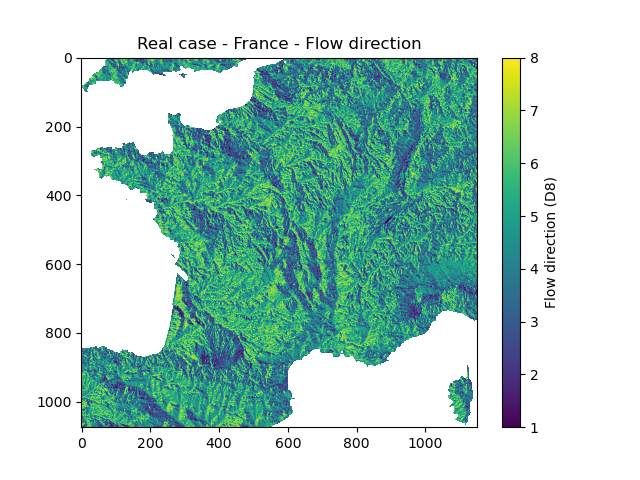
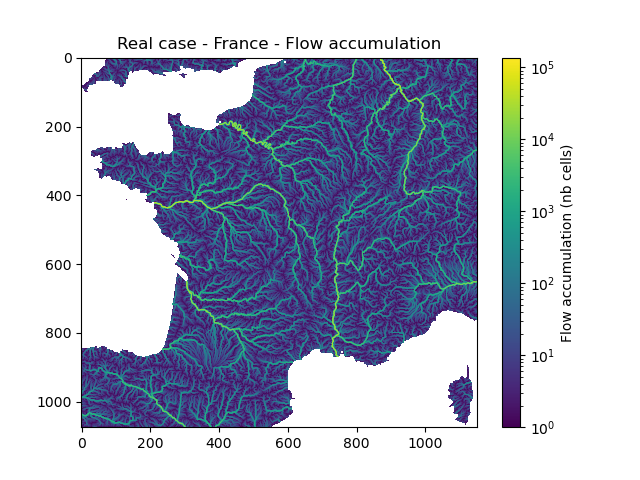
We can still visualize the extent of the grid, the flow directions and flow accumulation.

In [8]: mesh["nrow"], mesh["ncol"]
Out[8]: (1075, 1150)

In [9]: plt.imshow(mesh["flwdir"]);

In [10]: plt.colorbar(label="Flow direction (D8)");

In [11]: plt.title("Real case - France - Flow direction");

In [12]: plt.imshow(mesh["flwacc"], norm=LogNorm());

In [13]: plt.colorbar(label="Flow accumulation (nb cells)");

In [14]: plt.title("Real case - France - Flow accumulation");

This mesh can also be automatically generated by providing to the smash.generate_mesh() method the France flow directions and the bouding box (xmin, xmax, ymin, ymax).

In [15]: flwdir = smash.load_dataset("flwdir")

In [16]: france_bbox = (100_000, 1_250_000, 6_050_000, 7_125_000)

In [17]: mesh2 = smash.generate_mesh(
   ....:     path=flwdir,
   ....:     bbox=france_bbox
   ....: )
   ....: 

This mesh2 created is a dictionnary which is identical to the mesh loaded with the smash.load_dataset() method.

In [18]: mesh2["nrow"], mesh2["ncol"]
Out[18]: (1075, 1150)

Finally, create the smash.Model object using the setup and mesh loaded.

In [19]: model = smash.Model(setup, mesh)

In [20]: model
Out[20]: 
Structure: 'gr-a'
Spatio-Temporal dimension: (x: 1150, y: 1075, time: 32)
Last update: Initialization

Run

Forward run

Make a forward run using the Model.run() method.

In [21]: model.run(inplace=True);

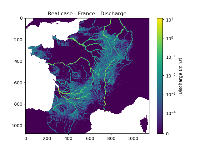
We can visualize the simulated discharges after a forward run on the whole domain. Here for the last time step of simulation.

In [22]: qsim = model.output.qsim_domain[..., -1]

In [23]: qsim = np.where(model.mesh.active_cell == 0, np.nan, qsim)

In [24]: plt.imshow(qsim, norm=SymLogNorm(1e-4));

In [25]: plt.colorbar(label="Discharge $(m^3/s)$");

In [26]: plt.title("Real case - France - Discharge");

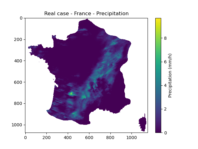
We can visualize the precipitation for the same time step. In addition to masking the non active cells, we mask the cells where there is no precipitation data (i.e. precipitation lower than 0).

In [27]: prcp = model.input_data.prcp[..., -1]

In [28]: prcp = np.where(
   ....:     np.logical_or(model.mesh.active_cell == 0, prcp < 0),
   ....:     np.nan,
   ....:     prcp
   ....: )
   ....: 

In [29]: plt.imshow(prcp);

In [30]: plt.colorbar(label="Precipitation (mm/h)");

In [31]: plt.title("Real case - France - Precipitation");