Real case - Cance#
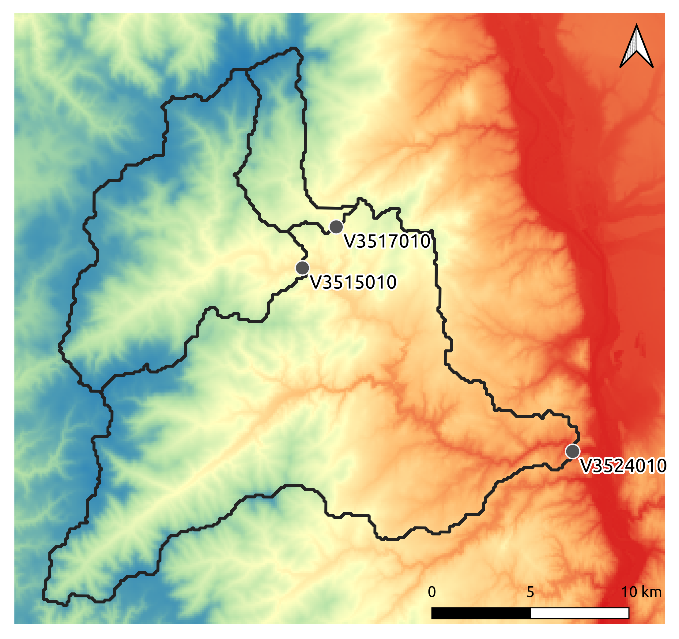
A real case is considered: the Cance river catchment at Sarras, a right bank tributary of the Rhône river.
First, open a Python interface:
python3
Imports#
In [1]: import smash

In [2]: import numpy as np

In [3]: import matplotlib.pyplot as plt
Model object creation#
Creating a Model requires two input arguments: setup and mesh. For this case, it is possible to directly load the both input dictionnaries using the smash.load_dataset() method.
In [4]: setup, mesh = smash.load_dataset("Cance")
Setup argument#
setup is a dictionary that allows to initialize Model (i.e. allocate the necessary Fortran arrays).
Note
Each key and associated values that can be passed into the setup dictionary are detailed in the User Guide section: Model initialization.
Compared to the Practice case, more options have been filled in the setup dictionary.
In [5]: setup
Out[5]:
{'structure': 'gr-a',
 'dt': 3600,
 'start_time': '2014-09-15 00:00',
 'end_time': '2014-11-14 00:00',
 'read_qobs': True,
 'qobs_directory': '/home/fcolleoni/anaconda3/envs/smash-dev/lib/python3.11/site-packages/smash/dataset/Cance/qobs',
 'read_prcp': True,
 'prcp_format': 'tif',
 'prcp_conversion_factor': 0.1,
 'prcp_directory': '/home/fcolleoni/anaconda3/envs/smash-dev/lib/python3.11/site-packages/smash/dataset/Cance/prcp',
 'read_pet': True,
 'pet_format': 'tif',
 'pet_conversion_factor': 1,
 'daily_interannual_pet': True,
 'pet_directory': '/home/fcolleoni/anaconda3/envs/smash-dev/lib/python3.11/site-packages/smash/dataset/Cance/pet',
 'read_descriptor': True,
 'descriptor_name': ['slope', 'dd'],
 'descriptor_directory': '/home/fcolleoni/anaconda3/envs/smash-dev/lib/python3.11/site-packages/smash/dataset/Cance/descriptor'}
To get into the details:
structure: the model structure,dt: the calculation time step in s,start_time: the beginning of the simulation,end_time: the end of the simulation,read_qobs: whether or not to read observed discharges files,qobs_directory: the path to the observed discharges files (this path is automatically generated when you load the data),read_prcp: whether or not to read precipitation files,prcp_format: the precipitation files format (tifformat is the only available at the moment),prcp_conversion_factor: the precipitation conversion factor (the precipitation value will be multiplied by the conversion factor),prcp_directory: the path to the precipitation files (this path is automatically generated when you load the data),read_pet: whether or not to read potential evapotranspiration files,pet_format: the potential evapotranspiration files format (tifformat is the only available at the moment),pet_conversion_factor: the potential evapotranspiration conversion factor (the potential evapotranspiration value will be multiplied by the conversion factor),daily_interannual_pet: whether or not to read potential evapotranspiration files as daily interannual value desaggregated to the corresponding time stepdt,pet_directory: the path to the potential evapotranspiration files (this path is automatically generated when you load the data),read_descriptor: whether or not to read catchment descriptors files,descriptor_name: the names of the descriptors (the name must correspond to the name of the file without the extension such asslope.tif),descriptor_directory: the path to the catchment descriptors files (this path is automatically generated when you load the data),
Note
See the User Guide section: Model structure for more information about model structure
See the User Guide section: Model input data convention for more information about model input data convention
Mesh argument#
Mesh composition#
mesh is a dictionary that allows to initialize Model (i.e. allocate the necessary Fortran arrays).
Note
Each key and associated values that can be passed into the mesh dictionary are detailed in the User Guide section: Model initialization.
In [6]: mesh.keys()
Out[6]: dict_keys(['dx', 'nac', 'ncol', 'ng', 'nrow', 'xmin', 'ymax', 'active_cell', 'area', 'code', 'flwacc', 'flwdir', 'flwdst', 'gauge_pos', 'path'])
To get into the details:
dx: the calculation spatial step in m,
In [7]: mesh["dx"]
Out[7]: 1000.0
xmin: the minimum value of the domain extension in x (it depends on the flow directions projection)
In [8]: mesh["xmin"]
Out[8]: 813000.0
ymax: the maximum value of the domain extension in y (it depends on the flow directions projection)
In [9]: mesh["ymax"]
Out[9]: 6478000.0
nrow: the number of rows,
In [10]: mesh["nrow"]
Out[10]: 28
ncol: the number of columns,
In [11]: mesh["ncol"]
Out[11]: 28
ng: the number of gauges,
In [12]: mesh["ng"]
Out[12]: 3
nac: the number of cells that contribute to any gauge discharge,
In [13]: mesh["nac"]
Out[13]: 383
area: the catchments area in m²,
In [14]: mesh["area"]
Out[14]: array([3.83e+08, 1.08e+08, 2.80e+07], dtype=float32)
code: the gauges code,
In [15]: mesh["code"]
Out[15]: array(['V3524010', 'V3515010', 'V3517010'], dtype='<U8')
gauge_pos: the gauges position in the grid,
In [16]: mesh["gauge_pos"]
Out[16]:
array([[20, 27],
       [10, 13],
       [ 8, 14]], dtype=int32)
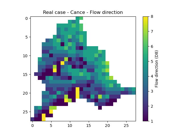
flwdir: the flow directions,
In [17]: plt.imshow(mesh["flwdir"]);

In [18]: plt.colorbar(label="Flow direction (D8)");

In [19]: plt.title("Real case - Cance - Flow direction");
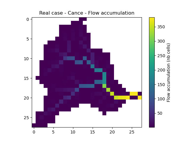
flwacc: the flow accumulation in number of cells,
In [20]: plt.imshow(mesh["flwacc"]);

In [21]: plt.colorbar(label="Flow accumulation (nb cells)");

In [22]: plt.title("Real case - Cance - Flow accumulation");
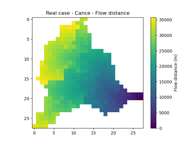
flwdst: the flow distances from the main outlet in m,
In [23]: plt.imshow(mesh["flwdst"]);

In [24]: plt.colorbar(label="Flow distance (m)");

In [25]: plt.title("Real case - Cance - Flow distance");
active_cell: the cells that contribute to any gauge discharge (mask),
In [26]: plt.imshow(mesh["active_cell"]);

In [27]: plt.colorbar(label="Logical active cell (0: False, 1: True)");

In [28]: plt.title("Real case - Cance - Active cell");

path: the calculation path.
In [29]: mesh["path"]
Out[29]:
array([[13, 16, 16, ..., 19, 19, 20],
       [27, 21, 19, ..., 25, 26, 27]], dtype=int32)
Obviously, the data set included in the mesh dictionary is not generated by hand. The method smash.generate_mesh() allows from a flow directions file, the gauge coordinates and the area to generate this same data set. More details can be found in the User Guide section: Automatic meshing.
Generate a mesh automatically#
The method required the path to the flow directions tif file. One can load it directly with,
In [30]: flwdir = smash.load_dataset("flwdir")

In [31]: flwdir
Out[31]: '/home/fcolleoni/anaconda3/envs/smash-dev/lib/python3.11/site-packages/smash/dataset/France_flwdir.tif'
This path leads to a flow directions tif file of the whole France at 1km spatial resolution and Lambert93 projection (EPSG:2154)
Get the gauge coordinates, area and code (this data is considered to be known by the user at the time the mesh is generated):
In [32]: x = [840_261, 826_553, 828_269]

In [33]: y = [6_457_807, 6_467_115, 6_469_198]

In [34]: area = [381.7 * 1e6, 107 * 1e6, 25.3 * 1e6]

In [35]: code = ["V3524010", "V3515010", "V3517010"]
The x and y coordinates of the gauge must be in the same projection of the flow directions used for the meshing, here Lambert93 (EPSG:2154). The area must be in m².
Call the smash.generate_mesh() method:
In [36]: mesh2 = smash.generate_mesh(
   ....:     path=flwdir,
   ....:     x=x,
   ....:     y=y,
   ....:     area=area,
   ....:     code=code,
   ....: )
   ....:
This mesh2 created is a dictionnary which is identical to the mesh loaded with the smash.load_dataset() method.
In [37]: mesh2["dx"], mesh2["nrow"], mesh2["ncol"], mesh2["ng"], mesh2["gauge_pos"]
Out[37]:
(1000.0,
 28,
 28,
 3,
 array([[20, 27],
        [10, 13],
        [ 8, 14]], dtype=int32))
As a remainder, the mesh can be saved to HDF5 using the smash.save_mesh() method and reload with the smash.read_mesh() method.
In [38]: smash.save_mesh(mesh2, "mesh_Cance.hdf5")

In [39]: mesh3 = smash.read_mesh("mesh_Cance.hdf5")

In [40]: mesh3["dx"], mesh3["nrow"], mesh3["ncol"], mesh3["ng"], mesh3["gauge_pos"]
Out[40]:
(1000.0,
 28,
 28,
 3,
 array([[20, 27],
        [10, 13],
        [ 8, 14]], dtype=int32))
Finally, create the Model object using the setup and mesh loaded.
In [41]: model = smash.Model(setup, mesh)

In [42]: model
Out[42]:
Structure: 'gr-a'
Spatio-Temporal dimension: (x: 28, y: 28, time: 1440)
Last update: Initialization
Viewing Model#
Similar to the Practice case, it is possible to visualize what the Model contains through the 6 attributes: Model.setup, Model.mesh, Model.input_data,
Model.parameters, Model.states, Model.output. As we have already detailed in the Practice case the access to any data, we will only visualize the observed discharges and the spatialized atmospheric forcings here.
Input Data - Observed discharge#
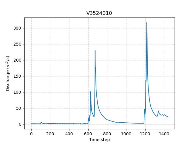
3 gauges were placed in the meshing. For the sake of clarity, only the most downstream gauge discharge V3524010 is plotted.
In [43]: plt.plot(model.input_data.qobs[0,:]);

In [44]: plt.grid(alpha=.7, ls="--");

In [45]: plt.xlabel("Time step");

In [46]: plt.ylabel("Discharge ($m^3/s$)");

In [47]: plt.title(model.mesh.code[0]);
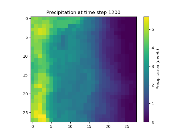
Input Data - Atmospheric forcings#
Precipitation and potential evapotranspiration files were read for each time step. For the sake of clarity, only one precipiation grid at time step 1200 is plotted.
In [48]: plt.imshow(model.input_data.prcp[..., 1200]);

In [49]: plt.title("Precipitation at time step 1200");

In [50]: plt.colorbar(label="Precipitation ($mm/h$)");
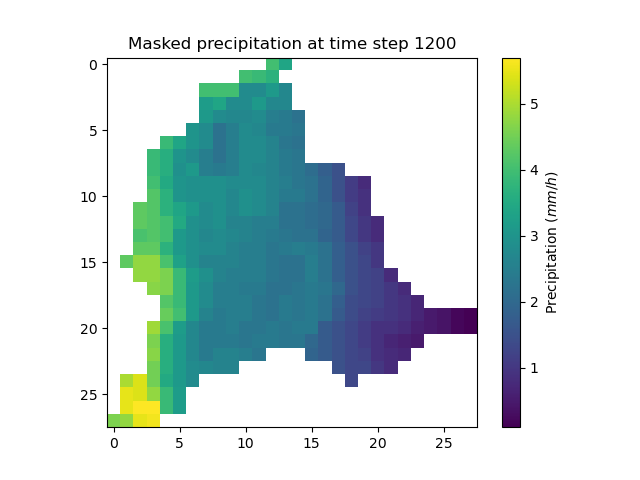
It is possible to mask the precipitation grid to only visualize the precipitation on active cells using numpy method np.where.
In [51]: ma_prcp = np.where(
   ....:     model.mesh.active_cell == 0,
   ....:     np.nan,
   ....:     model.input_data.prcp[..., 1200]
   ....: )
   ....:

In [52]: plt.imshow(ma_prcp);

In [53]: plt.title("Masked precipitation at time step 1200");

In [54]: plt.colorbar(label="Precipitation ($mm/h$)");
Run#
Forward run#
Make a forward run using the Model.run() method.
In [55]: model.run();
Here, unlike the Practice case, we have not specified inplace=True. By default, this argument is assigned to False, i.e. when the Model.run() method is called, the model object is not modified in-place but in a copy which can be returned.
So if we display the representation of the model, the last update will still be Initialization and no simulated discharge is available.
In [56]: model
Out[56]:
Structure: 'gr-a'
Spatio-Temporal dimension: (x: 28, y: 28, time: 1440)
Last update: Initialization

In [57]: model.output.qsim
Out[57]:
array([[-99., -99., -99., ..., -99., -99., -99.],
       [-99., -99., -99., ..., -99., -99., -99.],
       [-99., -99., -99., ..., -99., -99., -99.]], dtype=float32)
This argument is useful to keep the original Model and store the results of the forward run in an other instance.
In [58]: model_forward = model.run();

In [59]: model
Out[59]:
Structure: 'gr-a'
Spatio-Temporal dimension: (x: 28, y: 28, time: 1440)
Last update: Initialization

In [60]: model_forward
Out[60]:
Structure: 'gr-a'
Spatio-Temporal dimension: (x: 28, y: 28, time: 1440)
Last update: Forward Run
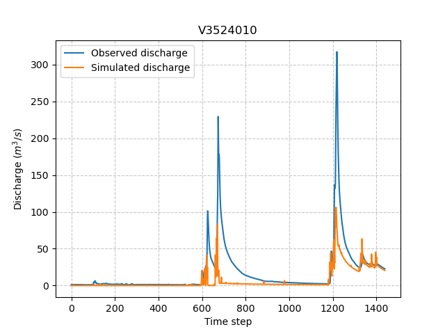
We can visualize the simulated discharges after a forward run for the most downstream gauge.
In [61]: plt.plot(model_forward.input_data.qobs[0,:], label="Observed discharge");

In [62]: plt.plot(model_forward.output.qsim[0,:], label="Simulated discharge");

In [63]: plt.grid(alpha=.7, ls="--");

In [64]: plt.xlabel("Time step");

In [65]: plt.ylabel("Discharge $(m^3/s)$");

In [66]: plt.title(model_forward.mesh.code[0]);

In [67]: plt.legend();
Optimization#
Let us briefly formulate here the general hydrological model calibration inverse problem. Let \(J \left( \theta \right)\) be a cost function measuring the misfit between simulated and observed quantities, such as discharge. Note that \(J\) depends on the sought parameter set \(\theta\) throught the hydrological model \(\mathcal{M}\). An optimal estimate of \(\hat{\theta}\) of model parameter set is obtained from the condition:
Several calibration strategies are available in smash. They are based on different optimization algorithms and are for example adapted to inverse problems of various complexity, including high dimensional ones.
For the purposes of the User Guide, we will only perform a spatially uniform and distributed optimization on the most downstream gauge.
Spatially uniform optimization#
We consider here for optimization (which is the default setup with gr-a structure):
a global minimization algorithm \(\mathrm{SBS}\),
a single \(\mathrm{NSE}\) objective function from discharge time series at the most downstream gauge
V3524010,a spatially uniform parameter set \(\theta = \left( \mathrm{cp, cft, lr, exc} \right)^T\) with \(\mathrm{cp}\) being the maximum capacity of the production reservoir, \(\mathrm{cft}\) being the maximum capacity of the transfer reservoir, \(\mathrm{lr}\) being the linear routing parameter and \(\mathrm{exc}\) being the non-conservative exchange parameter.
Call the Model.optimize() method and for the sake of computation time, set the maximum number of iterations in the options argument to 2.
In [68]: model_su = model.optimize(options={"maxiter": 2});
While the optimization routine is in progress, some information are provided.
</> Optimize Model J
    Mapping: 'uniform' k(X)
    Algorithm: 'sbs'
    Jobs function: [ nse ]
    wJobs: [ 1.0 ]
    Nx: 1
    Np: 4 [ cp cft exc lr ]
    Ns: 0 [  ]
    Ng: 1 [ V3524010 ]
    wg: 1 [ 1.0 ]

    At iterate      0    nfg =     1    J =  0.677404    ddx = 0.64
    At iterate      1    nfg =    30    J =  0.130012    ddx = 0.64
    At iterate      2    nfg =    59    J =  0.043658    ddx = 0.32
    STOP: TOTAL NO. OF ITERATION EXCEEDS LIMIT
This information remainds the ptimization options:
Mapping: the optimization mapping of parameters,Algorithm: the minimization algorithm,Jobs_fun: the objective function(s),wJobs: the weight assigned to each objective function,Nx: the dimension of the problem (1 means that we perform a spatially uniform optimization),Np: the number of parameters to optimize and their name,Ns: the number of initial states to optimize and their name,Ng: the number of gauges to optimize and their code/name,wg: the weight assigned to each optimized gauge.
Note
The size of the control vector is defined by \(Nx \left(Np + Ns \right)\)
Then, for each iteration, we can retrieve:
nfg: the total number of function and gradient evaluations (there is no gradient evaluations in the minimization algorithm \(\mathrm{SBS}\)),J: the value of the cost function,ddx: the convergence criterion specific to the minimization algorithm \(\mathrm{SBS}\) (the algorithm converges whenddxis lower than 0.01).
The last line informs about the reason why the optimization ended. Here, since we have forced 2 iterations maximum, the algorithm stopped because the number of iterations was exceeded.
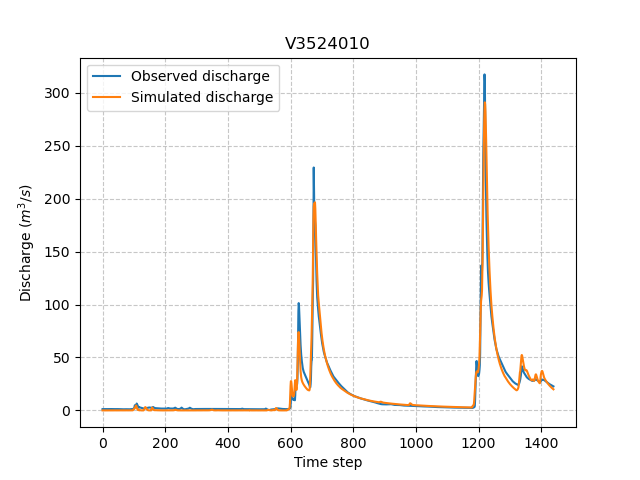
Once the optimization is complete. We can visualize the simulated discharge,
In [69]: plt.plot(model_su.input_data.qobs[0,:], label="Observed discharge");

In [70]: plt.plot(model_su.output.qsim[0,:], label="Simulated discharge");

In [71]: plt.grid(alpha=.7, ls="--");

In [72]: plt.xlabel("Time step");

In [73]: plt.ylabel("Discharge $(m^3/s)$");

In [74]: plt.title(model_su.mesh.code[0]);

In [75]: plt.legend();
The cost function value \(J\) (should be equal to the last iteration J),
In [76]: model_su.output.cost
Out[76]: 0.04365839809179306
The optimized parameters \(\hat{\theta}\) (for the sake of clarity and because we performed a spatially uniform optimization, we will only display the parameter set values for one cell within the catchment active cells, which is the most downstream gauge position here),
In [77]: ind = tuple(model_su.mesh.gauge_pos[0,:])

In [78]: ind
Out[78]: (20, 27)

In [79]: (
   ....:  model_su.parameters.cp[ind],
   ....:  model_su.parameters.cft[ind],
   ....:  model_su.parameters.lr[ind],
   ....:  model_su.parameters.exc[ind],
   ....: )
   ....:
Out[79]: (76.57858, 263.64627, 34.10478, -0.6845942)
Spatially distributed optimization#
We consider here for optimization:
a gradient descent minimization algorithm \(\mathrm{L}\text{-}\mathrm{BFGS}\text{-}\mathrm{B}\),
a single \(\mathrm{NSE}\) objective function from discharge time series at the most downstream gauge
V3524010,a spatially distributed parameter set \(\theta = \left( \mathrm{cp, cft, lr, exc} \right)^T\) with \(\mathrm{cp}\) being the maximum capacity of the production reservoir, \(\mathrm{cft}\) being the maximum capacity of the transfer reservoir, \(\mathrm{lr}\) being the linear routing parameter and \(\mathrm{exc}\) being the non-conservative exchange parameter.
a prior set of parameters \(\bar{\theta}^*\) generated from the previous spatially uniform global optimization.
Call the Model.optimize() method, fill in the arguments mapping with “distributed” and for the sake of computation time, set the maximum number of iterations in the options argument to 15.
As we run this optimization from the previously generated uniform parameter set, we apply the Model.optimize() method from the model_su instance which had stored the previous optimized parameters.
In [80]: model_sd = model_su.optimize(
   ....:         mapping="distributed",
   ....:         options={"maxiter": 15}
   ....:     )
   ....:
While the optimization routine is in progress, some information are provided.
</> Optimize Model J
    Mapping: 'distributed' k(x)
    Algorithm: 'l-bfgs-b'
    Jobs function: [ nse ]
    wJobs: [ 1.0 ]
    Jreg function: 'prior'
    wJreg: 0.000000
    Nx: 383
    Np: 4 [ cp cft exc lr ]
    Ns: 0 [  ]
    Ng: 1 [ V3524010 ]
    wg: 1 [ 1.0 ]

    At iterate      0    nfg =     1    J =  0.043658    |proj g| =  0.000000
    At iterate      1    nfg =     3    J =  0.039536    |proj g| =  0.025741
    At iterate      2    nfg =     4    J =  0.039269    |proj g| =  0.010773
    At iterate      3    nfg =     5    J =  0.039050    |proj g| =  0.012686
    At iterate      4    nfg =     6    J =  0.038270    |proj g| =  0.031537
    At iterate      5    nfg =     7    J =  0.037304    |proj g| =  0.035111
    At iterate      6    nfg =     8    J =  0.036115    |proj g| =  0.029365
    At iterate      7    nfg =     9    J =  0.035208    |proj g| =  0.007301
    At iterate      8    nfg =    10    J =  0.034932    |proj g| =  0.015130
    At iterate      9    nfg =    11    J =  0.034774    |proj g| =  0.018046
    At iterate     10    nfg =    12    J =  0.034298    |proj g| =  0.013504
    At iterate     11    nfg =    13    J =  0.033304    |proj g| =  0.012190
    At iterate     12    nfg =    14    J =  0.031491    |proj g| =  0.014053
    At iterate     13    nfg =    15    J =  0.029747    |proj g| =  0.012535
    At iterate     14    nfg =    16    J =  0.028294    |proj g| =  0.031778
    At iterate     15    nfg =    18    J =  0.027901    |proj g| =  0.003941
    STOP: TOTAL NO. OF ITERATION EXCEEDS LIMIT
The information are broadly similar to the spatially uniform optimization, except for
Jreg_function: the regularization function,wJreg: the weight assigned to the regularization term,
Note
We did not specified any regularization options. Therefore, the wJreg term is set to 0 and no regularization is applied to the optimization.
Then, for each iteration, we can retrieve same information with nfg (there are gradients evaluations for the \(\mathrm{L}\text{-}\mathrm{BFGS}\text{-}\mathrm{B}\) algorithm) and J.
|proj g| is the infinity norm of the projected gradient.
Note
The cost function \(J\) at 0th iteration is equal to the cost function at the end of the spatially uniform optimization. This means that we used the previous optimized parameters as new prior.
The algorithm also stopped because the number of iterations was exceeded.
We can once again visualize, the simulated discharges (su: spatially uniform, sd: spatially distributed)
In [81]: plt.plot(model_sd.input_data.qobs[0,:], label="Observed discharge");

In [82]: plt.plot(model_su.output.qsim[0,:], label="Simulated discharge - su");

In [83]: plt.plot(model_sd.output.qsim[0,:], label="Simulated discharge - sd");

In [84]: plt.grid(alpha=.7, ls="--");

In [85]: plt.xlabel("Time step");

In [86]: plt.ylabel("Discharge $(m^3/s)$");

In [87]: plt.title(model_sd.mesh.code[0]);

In [88]: plt.legend();
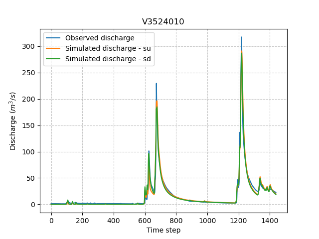
Note
The difference between the two simulated discharges is very slight. Indeed, the spatially uniform optimization already leads to rather good performances with a cost function \(J\) equal to 0.04. Spatially distributed optimization only improved the performances by approximately 0.02.
The cost function value \(J\),
In [89]: model_sd.output.cost
Out[89]: 0.027900615707039833
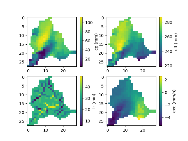
The optimized parameters \(\hat{\theta}\),
In [90]: ma = (model_sd.mesh.active_cell == 0)

In [91]: ma_cp = np.where(ma, np.nan, model_sd.parameters.cp)

In [92]: ma_cft = np.where(ma, np.nan, model_sd.parameters.cft)

In [93]: ma_lr = np.where(ma, np.nan, model_sd.parameters.lr)

In [94]: ma_exc = np.where(ma, np.nan, model_sd.parameters.exc)

In [95]: f, ax = plt.subplots(2, 2)

In [96]: map_cp = ax[0,0].imshow(ma_cp);

In [97]: f.colorbar(map_cp, ax=ax[0,0], label="cp (mm)");

In [98]: map_cft = ax[0,1].imshow(ma_cft);

In [99]: f.colorbar(map_cft, ax=ax[0,1], label="cft (mm)");

In [100]: map_lr = ax[1,0].imshow(ma_lr);

In [101]: f.colorbar(map_lr, ax=ax[1,0], label="lr (min)");

In [102]: map_exc = ax[1,1].imshow(ma_exc);

In [103]: f.colorbar(map_exc, ax=ax[1,1], label="exc (mm/h)");
Getting data#
Finally and as a remainder of the Practice case, it is possible to save any Model object to HDF5. Here, we will save both optimized instances.
In [104]: smash.save_model(model_su, "su_optimize_Cance.hdf5")

In [105]: smash.save_model(model_sd, "sd_optimize_Cance.hdf5")
And reload them as follows
In [106]: model_su_reloaded = smash.read_model("su_optimize_Cance.hdf5")

In [107]: model_sd_reloaded = smash.read_model("sd_optimize_Cance.hdf5")

In [108]: model_su, model_su_reloaded
Out[108]:
(Structure: 'gr-a'
 Spatio-Temporal dimension: (x: 28, y: 28, time: 1440)
 Last update: SBS Optimization,
 Structure: 'gr-a'
 Spatio-Temporal dimension: (x: 28, y: 28, time: 1440)
 Last update: SBS Optimization)

In [109]: model_sd, model_sd_reloaded
Out[109]:
(Structure: 'gr-a'
 Spatio-Temporal dimension: (x: 28, y: 28, time: 1440)
 Last update: L-BFGS-B Optimization,
 Structure: 'gr-a'
 Spatio-Temporal dimension: (x: 28, y: 28, time: 1440)
 Last update: L-BFGS-B Optimization)