Event segmentation

This section aims to go into detail on how to use and visualize the hydrograph segmentation from a proposed algorithm as depicted in section Math / Num Documentation.

First, open a Python interface:

python3

Imports

In [1]: import smash

In [2]: import matplotlib.pyplot as plt

In [3]: import pandas as pd

Model object creation

To obtain flood events segmentation, you need to create a smash.Model object. For this case, we will use the Cance dataset used in the User Guide section: Real case - Cance.

Load the setup and mesh dictionaries using the smash.load_dataset() method and create the smash.Model object.

In [4]: setup, mesh = smash.load_dataset("Cance")

In [5]: model = smash.Model(setup, mesh)

Flood event information and visualization

Once the smash.Model object is created, the flood events information are available using the Model.event_segmentation() method.

In [6]: event_seg = model.event_segmentation();

In [7]: event_seg
Out[7]: 
       code               start                 end         maxrainfall               flood  season
0  V3524010 2014-11-03 03:00:00 2014-11-10 12:00:00 2014-11-04 12:00:00 2014-11-04 19:00:00  autumn
1  V3515010 2014-11-03 10:00:00 2014-11-10 11:00:00 2014-11-04 12:00:00 2014-11-04 20:00:00  autumn
2  V3517010 2014-11-03 08:00:00 2014-11-10 23:00:00 2014-11-04 11:00:00 2014-11-04 16:00:00  autumn

The result is represented by a pandas.DataFrame with 6 columns.

• code : The catchment code,

• start : The beginning of event under YYYY-MM-DD HH:MM:SS format,

• end : The end of event under YYYY-MM-DD HH:MM:SS format,

• maxrainfall : The moment when the maximum precipation is observed under YYYY-MM-DD HH:MM:SS format,

• flood : The moment when the maximum discharge is observed under YYYY-MM-DD HH:MM:SS format,

• season : The season in which the event occurs.

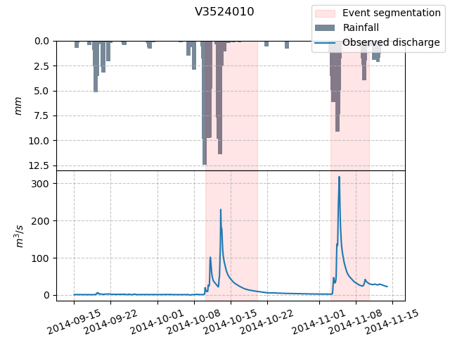
Then the segmented event, for instance of catchment V3524010, is shown in the hydrograph below.

In [8]: dti = pd.date_range(start=model.setup.start_time, end=model.setup.end_time, freq="H")[1:]

In [9]: qo = model.input_data.qobs[0, :]

In [10]: prcp = model.input_data.mean_prcp[0, :]

In [11]: starts = pd.to_datetime(event_seg["start"])

In [12]: ends = pd.to_datetime(event_seg["end"])

In [13]: fig, (ax1, ax2) = plt.subplots(2, 1)

In [14]: fig.subplots_adjust(hspace=0)

In [15]: ax1.bar(dti, prcp, color="lightslategrey", label="Rainfall");

In [16]: ax1.axvspan(starts[0], ends[0], alpha=.1, color="red", label="Event segmentation");

In [17]: ax1.grid(alpha=.7, ls="--")

In [18]: ax1.get_xaxis().set_visible(False)

In [19]: ax1.set_ylabel("$mm$");

In [20]: ax1.invert_yaxis()

In [21]: ax2.plot(dti, qo, label="Observed discharge");

In [22]: ax2.axvspan(starts[0], ends[0], alpha=.1, color="red");

In [23]: ax2.grid(alpha=.7, ls="--")

In [24]: ax2.tick_params(axis="x", labelrotation=20)

In [25]: ax2.set_ylabel("$m^3/s$");

In [26]: ax2.set_xlim(ax1.get_xlim());

In [27]: fig.legend();

In [28]: fig.suptitle("V3524010");

In this case, an event seems to be missing but we can always adjust some parameters of the segmentation algorithm to detect flood events, for example:

In [29]: event_seg_2 = model.event_segmentation(peak_quant=0.99);

In [30]: event_seg_2
Out[30]: 
       code               start                 end         maxrainfall               flood  season
0  V3524010 2014-10-10 04:00:00 2014-10-20 03:00:00 2014-10-12 23:00:00 2014-10-13 02:00:00  autumn
1  V3524010 2014-11-03 03:00:00 2014-11-10 12:00:00 2014-11-04 12:00:00 2014-11-04 19:00:00  autumn
2  V3515010 2014-10-10 04:00:00 2014-10-19 20:00:00 2014-10-10 20:00:00 2014-10-13 00:00:00  autumn
3  V3515010 2014-11-03 10:00:00 2014-11-10 11:00:00 2014-11-04 12:00:00 2014-11-04 20:00:00  autumn
4  V3517010 2014-10-09 15:00:00 2014-10-19 22:00:00 2014-10-10 20:00:00 2014-10-10 23:00:00  autumn
5  V3517010 2014-11-03 08:00:00 2014-11-10 23:00:00 2014-11-04 11:00:00 2014-11-04 16:00:00  autumn

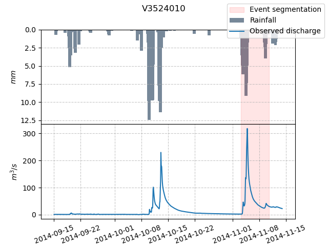
We can once again visualize, the segmented events of catchment V3524010 on the hydrograph.

In [31]: starts = pd.to_datetime(event_seg_2["start"])

In [32]: ends = pd.to_datetime(event_seg_2["end"])

In [33]: fig, (ax1, ax2) = plt.subplots(2, 1)

In [34]: fig.subplots_adjust(hspace=0)

In [35]: ax1.bar(dti, prcp, color="lightslategrey", label="Rainfall");

In [36]: ax1.axvspan(starts[0], ends[0], alpha=.1, color="red", label="Event segmentation");

In [37]: ax1.axvspan(starts[1], ends[1], alpha=.1, color="red");

In [38]: ax1.grid(alpha=.7, ls="--")

In [39]: ax1.get_xaxis().set_visible(False)

In [40]: ax1.set_ylabel("$mm$");

In [41]: ax1.invert_yaxis()

In [42]: ax2.plot(dti, qo, label="Observed discharge");

In [43]: ax2.axvspan(starts[0], ends[0], alpha=.1, color="red");

In [44]: ax2.axvspan(starts[1], ends[1], alpha=.1, color="red");

In [45]: ax2.grid(alpha=.7, ls="--")

In [46]: ax2.tick_params(axis="x", labelrotation=20)

In [47]: ax2.set_ylabel("$m^3/s$");

In [48]: ax2.set_xlim(ax1.get_xlim());

In [49]: fig.legend();

In [50]: fig.suptitle("V3524010");