Signatures

This section aims to go into detail on how to compute and vizualize some hydrological signatures (a list of studied signatures and their formula is given in Math / Num Documentation) as well as the sensitivity of the model parameters to these signatures.

First, open a Python interface:

python3

Imports

In [1]: import smash

In [2]: import pandas as pd

Model object creation

To compute the signatures, you need to create a smash.Model object. For this case, we will use the Cance dataset used in the User Guide section: Real case - Cance.

Load the setup and mesh dictionaries using the smash.load_dataset() method and create the smash.Model object.

In [3]: setup, mesh = smash.load_dataset("Cance")

In [4]: model = smash.Model(setup, mesh)

Signatures computation

To start with, we need to run a direct (or optimized) simulation. Then the signatures computation result is available using the Model.signatures() method. The argument event_seg (only related to flood event signatures) could be defined for tuning the parameters of the segmentation algorithm.

In [5]: model.run(inplace=True);

In [6]: res = model.signatures(event_seg={"peak_quant": 0.99});

Hint

See the Model.event_segmentation() method, detailed in User Guide, for tuning the segmentation parameters.

The signatures computation result is represented as a smash.SignResult object containning 2 attributes which are 2 different dictionaries:

• cont : Continuous signatures computation result,

• event: Flood event signatures computation result.

Each dictionary has 2 keys which are 2 different pandas.DataFrame:

• obs: Observation result,

• sim: Simulation result.

For example, to display the simulated continuous signatures computation result.

In [7]: res.cont["sim"]
Out[7]: 
       code       Crc     Crchf     Crclf    Crch2r  Cfp2  Cfp10     Cfp50      Cfp90
0  V3524010  0.207456  0.070218  0.137234  0.338471   0.0    0.0  1.361164  26.941522
1  V3515010  0.138049  0.053059  0.084988  0.384347   0.0    0.0  0.101521   4.921440
2  V3517010  0.139057  0.052027  0.087028  0.374141   0.0    0.0  0.020496   1.314597

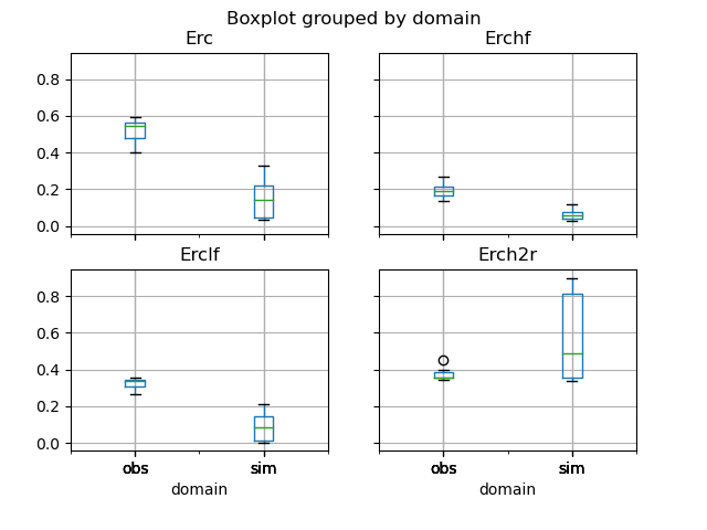
Now, we visualize, for instance, the simulated and observed flood event runoff coefficients in the boxplots below.

In [8]: df_obs = res.event["obs"]

In [9]: df_sim = res.event["sim"]

In [10]: df = pd.concat([df_obs, df_sim], ignore_index=True)

In [11]: df["domain"] = ["obs"]*len(df_obs) + ["sim"]*len(df_sim)

In [12]: boxplot = df.boxplot(column=["Erc", "Erchf", "Erclf", "Erch2r"], by="domain")

Signatures sensitivity

We are interested in investigating the variance-based sensitivities of the input model parameters to the output signatures. Several Sobol indices which are the first- and total-order sensitivities, are estimated using SALib Python library.

The problem argument can be defined if you prefer to change the default boundary constraints of the Model parameters. You can use the Model.get_bound_constraints() method to get the names of the Model parameters (depending on the defined Model structure) and its boundary constraints.

In [13]: model.get_bound_constraints()
Out[13]: 
{'num_vars': 4,
 'names': ['cp', 'cft', 'exc', 'lr'],
 'bounds': [[9.999999974752427e-07, 1000.0],
  [9.999999974752427e-07, 1000.0],
  [-50.0, 50.0],
  [9.999999974752427e-07, 1000.0]]}

Then you can redefine the problem to estimate the sensitivities of 3 parameters cp, cft, lr with the modified bounds (by fixing exc with its default value):

In [14]: problem = {
   ....:     "num_vars": 3,
   ....:     "names": ["cp", "cft", "lr"],
   ....:     "bounds": [[1,1000], [1,800], [1,500]]
   ....: }
   ....: 

The estimated sensitivities of the Model parameters to the signatures are available using the Model.signatures_sensitivity() method.

In [15]: res_sens = model.signatures_sensitivity(problem, n=16, event_seg={"peak_quant": 0.99}, random_state=99);

Note

In real-world applications, the value of n can be much larger to attain more accurate results.

Hint

See the Model.event_segmentation() method, detailed in User Guide, for tuning the segmentation parameters.

The signatures sensitivity result is represented as a smash.SignSensResult object containning 3 attributes which are 2 different dictionaries and 1 pandas.DataFrame:

• cont : Continuous signatures sensitivity result,

• event: Flood event signatures sensitivity result,

• sample: Generated samples used to estimate Sobol indices represented in a pandas.dataframe.

Each dictionary has 2 keys which are 2 different sub-dictionaries:

• total_si: Result of total-order sensitivities,

• first_si: Result of first-order sensitivities.

Each sub-dictionary has n_param keys (where n_param is the number of the model parameters), which are the dataframes containing the sensitivities of the associated model parameter to all studied signatures.

For example, to display the first-order sensitivities of the production parameter cp to all continuous signatures.

In [16]: res_sens.cont["first_si"]["cp"]
Out[16]: 
       code       Crc     Crchf     Crclf    Crch2r      Cfp2     Cfp10     Cfp50     Cfp90
0  V3524010  0.703305  0.273795  0.827588  0.040651  0.000747  0.266562  0.689595  0.630129
1  V3515010  0.646446  0.254117  0.816639  0.185909  0.012720  0.190930  0.607238  0.590940
2  V3517010  0.635774  0.268252  0.854603  0.368205  0.000272  0.070320  0.699551  0.805399

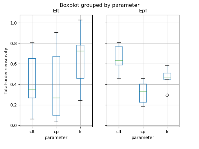
Finally, we visualize, for instance, the total-order sensitivities of the model parameters to the lag time Elt and the peak flow Epf.

In [17]: df_cp = res_sens.event["total_si"]["cp"]

In [18]: df_cft = res_sens.event["total_si"]["cft"]

In [19]: df_lr = res_sens.event["total_si"]["lr"]

In [20]: df_sens = pd.concat([df_cp, df_cft, df_lr], ignore_index=True)

In [21]: df_sens["parameter"] = ["cp"]*len(df_cp) + ["cft"]*len(df_cft) + ["lr"]*len(df_lr)

In [22]: boxplot_sens = df_sens.boxplot(column=["Elt", "Epf"], by="parameter")

In [23]: boxplot_sens[0].set_ylabel("Total-order sensitivity");