Hydrograph Segmentation#
This section provides a detailed guide on using and visualizing hydrograph segmentation based on the algorithm depicted in the Math / Num Documentation section.
First, open a Python interface:
python3
Imports#
We will first import the necessary libraries for this tutorial.
In [1]: import smash

In [2]: import matplotlib.pyplot as plt

In [3]: import pandas as pd
Model object creation#
Now, we need to create a smash.Model object.
For this case, we will use the Cance dataset as an example.
Load the setup and mesh dictionaries using the smash.factory.load_dataset function and create the smash.Model object.
In [4]: setup, mesh = smash.factory.load_dataset("Cance")

In [5]: model = smash.Model(setup, mesh)
</> Computing mean atmospheric data
</> Adjusting GR interception capacity
Flood event information and visualization#
Once the smash.Model object is created, the flood events information are available using the smash.hydrograph_segmentation function.
In [6]: event_seg = smash.hydrograph_segmentation(model);

In [7]: event_seg
Out[7]:
       code               start  ...               flood  season
0  V3524010 2014-11-03 03:00:00  ... 2014-11-04 19:00:00  autumn
1  V3515010 2014-11-03 10:00:00  ... 2014-11-04 20:00:00  autumn
2  V3517010 2014-11-03 08:00:00  ... 2014-11-04 16:00:00  autumn

[3 rows x 7 columns]

In [8]: event_seg.keys()
Out[8]: Index(['code', 'start', 'end', 'multipeak', 'maxrainfall', 'flood', 'season'], dtype='str')
The result is represented by a pandas.DataFrame with 7 columns.
code: The catchment code,start: The beginning of event underYYYY-MM-DD HH:MM:SSformat,end: The end of event underYYYY-MM-DD HH:MM:SSformat,multipeak: Boolean which indicates whether the event has multiple peaks,maxrainfall: The moment when the maximum precipitation is observed underYYYY-MM-DD HH:MM:SSformat,flood: The moment when the maximum discharge is observed underYYYY-MM-DD HH:MM:SSformat,season: The season in which the event occurs.
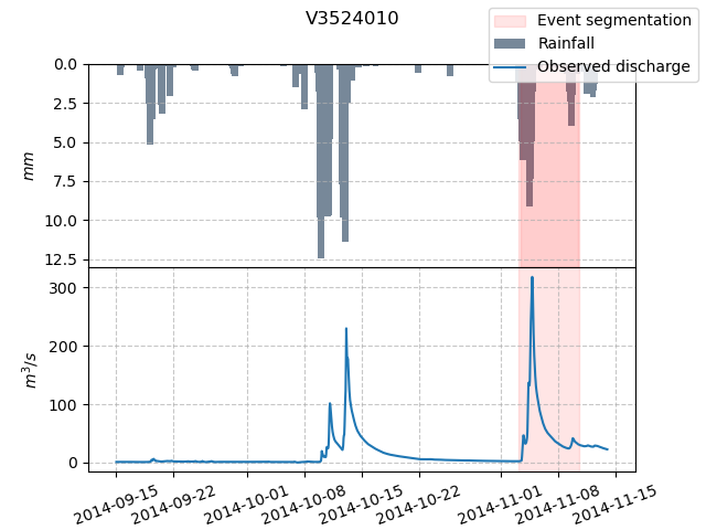
Then the segmented event, for instance of catchment V3524010, is shown in the hydrograph below.
In [9]: dti = pd.date_range(start=model.setup.start_time, end=model.setup.end_time, freq="h")[1:]

In [10]: qobs = model.response_data.q[0, :]

In [11]: mean_prcp = model.atmos_data.mean_prcp[0, :]

In [12]: starts = pd.to_datetime(event_seg["start"])

In [13]: ends = pd.to_datetime(event_seg["end"])

In [14]: fig, (ax1, ax2) = plt.subplots(2, 1)

In [15]: fig.subplots_adjust(hspace=0)

In [16]: ax1.bar(dti, mean_prcp, color="lightslategrey", label="Rainfall");

In [17]: ax1.axvspan(starts[0], ends[0], alpha=.1, color="red", label="Event segmentation");

In [18]: ax1.axvspan(starts[1], ends[1], alpha=.1, color="red");

In [19]: ax1.grid(alpha=.7, ls="--")

In [20]: ax1.get_xaxis().set_visible(False)

In [21]: ax1.set_ylabel("$mm$");

In [22]: ax1.invert_yaxis()

In [23]: ax2.plot(dti, qobs, label="Observed discharge");

In [24]: ax2.axvspan(starts[0], ends[0], alpha=.1, color="red");

In [25]: ax2.grid(alpha=.7, ls="--")

In [26]: ax2.tick_params(axis="x", labelrotation=20)

In [27]: ax2.set_ylabel("$m^3/s$");

In [28]: ax2.set_xlim(ax1.get_xlim());

In [29]: fig.legend();

In [30]: fig.suptitle("V3524010");
Customized flood event segmentation#
Several options are available to customize the flood event segmentation algorithm.
Quantile option#
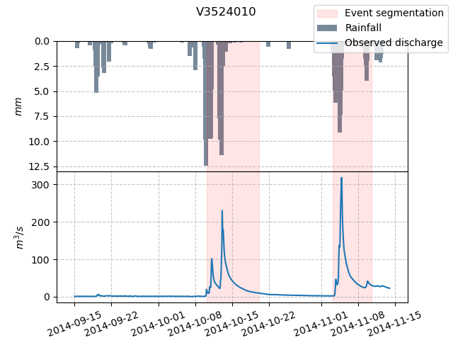
In the example above, an event seems to be missing. However, we can adjust the peak_quant parameter of the segmentation algorithm to detect more events.
By default, peak_quant is set to 0.995, meaning that only peaks exceeding the 0.995 quantile of the discharge are selected by the algorithm.
To detect more events, we can choose a smaller value, such as 0.99:
In [31]: event_seg_2 = smash.hydrograph_segmentation(model, peak_quant=0.99);

In [32]: event_seg_2
Out[32]:
       code               start  ...               flood  season
0  V3524010 2014-10-10 04:00:00  ... 2014-10-13 02:00:00  autumn
1  V3524010 2014-11-03 03:00:00  ... 2014-11-04 19:00:00  autumn
2  V3515010 2014-10-10 04:00:00  ... 2014-10-13 00:00:00  autumn
3  V3515010 2014-11-03 10:00:00  ... 2014-11-04 20:00:00  autumn
4  V3517010 2014-10-09 15:00:00  ... 2014-10-10 23:00:00  autumn
5  V3517010 2014-11-03 08:00:00  ... 2014-11-04 16:00:00  autumn

[6 rows x 7 columns]
We can once again visualize the segmented events of catchment V3524010 on the hydrograph, where a second event is now selected.
In [33]: starts = pd.to_datetime(event_seg_2["start"])

In [34]: ends = pd.to_datetime(event_seg_2["end"])

In [35]: fig, (ax1, ax2) = plt.subplots(2, 1)

In [36]: fig.subplots_adjust(hspace=0)

In [37]: ax1.bar(dti, mean_prcp, color="lightslategrey", label="Rainfall");

In [38]: ax1.axvspan(starts[0], ends[0], alpha=.1, color="red", label="Event segmentation");

In [39]: ax1.axvspan(starts[1], ends[1], alpha=.1, color="red");

In [40]: ax1.grid(alpha=.7, ls="--")

In [41]: ax1.get_xaxis().set_visible(False)

In [42]: ax1.set_ylabel("$mm$");

In [43]: ax1.invert_yaxis()

In [44]: ax2.plot(dti, qobs, label="Observed discharge");

In [45]: ax2.axvspan(starts[0], ends[0], alpha=.1, color="red");

In [46]: ax2.axvspan(starts[1], ends[1], alpha=.1, color="red");

In [47]: ax2.grid(alpha=.7, ls="--")

In [48]: ax2.tick_params(axis="x", labelrotation=20)

In [49]: ax2.set_ylabel("$m^3/s$");

In [50]: ax2.set_xlim(ax1.get_xlim());

In [51]: fig.legend();

In [52]: fig.suptitle("V3524010");
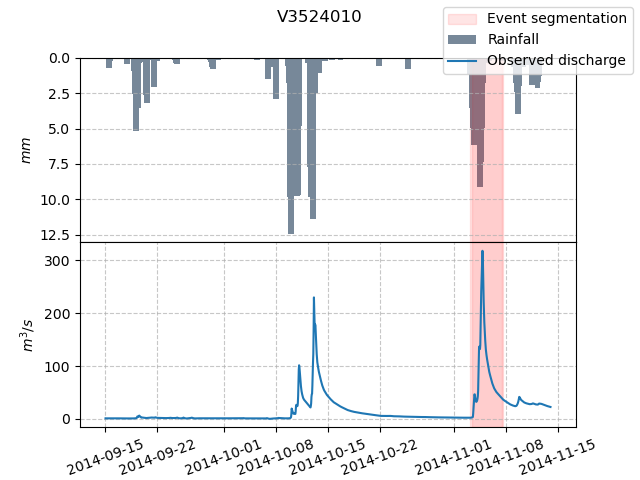
Threshold value option#
The threshold value to determine the peak of events can also be defined by the peak_value parameter.
By default, peak_value is set to 0 (not used). Once set, this parameter acts as a complementary criterion to peak_quant, meaning peaks must exceed both the quantile threshold and the specified value (in m³/s).
In [53]: event_seg_3 = smash.hydrograph_segmentation(model, peak_quant=0.99, peak_value=250);

In [54]: event_seg_3
Out[54]:
       code               start  ...               flood  season
0  V3524010 2014-11-03 03:00:00  ... 2014-11-04 19:00:00  autumn

[1 rows x 7 columns]
We can visualize the segmented events with the peak_value criterion applied:
In [55]: starts = pd.to_datetime(event_seg_3["start"])

In [56]: ends = pd.to_datetime(event_seg_3["end"])

In [57]: fig, (ax1, ax2) = plt.subplots(2, 1)

In [58]: fig.subplots_adjust(hspace=0)

In [59]: ax1.bar(dti, mean_prcp, color="lightslategrey", label="Rainfall");

In [60]: ax1.axvspan(starts[0], ends[0], alpha=.1, color="red", label="Event segmentation");

In [61]: ax1.grid(alpha=.7, ls="--")

In [62]: ax1.get_xaxis().set_visible(False)

In [63]: ax1.set_ylabel("$mm$");

In [64]: ax1.invert_yaxis()

In [65]: ax2.plot(dti, qobs, label="Observed discharge");

In [66]: ax2.axvspan(starts[0], ends[0], alpha=.1, color="red");

In [67]: ax2.axhline(y=250, color="orange", linestyle="--", label="Peak value threshold");

In [68]: ax2.grid(alpha=.7, ls="--")

In [69]: ax2.tick_params(axis="x", labelrotation=20)

In [70]: ax2.set_ylabel("$m^3/s$");

In [71]: ax2.set_xlim(ax1.get_xlim());

In [72]: fig.legend();

In [73]: fig.suptitle("V3524010");
Hint
To disable the peak quantile criterion and use only the peak_value criterion to select peaks, set peak_quant=0.
Gauge option#
The gauge parameter allows us to specify a list of catchment codes for which the hydrograph segmentation should be performed.
By default, the segmentation is applied to all catchments in the model. However, if we want to focus on specific catchments, we can provide them by either their codes or aliases.
# Only segment events for downstream gauge
In [74]: events_dws = smash.hydrograph_segmentation(model, gauge="dws");

In [75]: events_dws
Out[75]:
       code               start  ...               flood  season
0  V3524010 2014-11-03 03:00:00  ... 2014-11-04 19:00:00  autumn

[1 rows x 7 columns]
Max duration option#
The max_duration parameter sets the expected maximum duration of an event (in hours), which helps define the event end.
The default value is 240 hours, but it can be adjusted as needed. For example, setting max_duration=120 limits event durations to a maximum of 120 hours:
In [76]: event_seg_4 = smash.hydrograph_segmentation(model, max_duration=120);

In [77]: event_seg_4
Out[77]:
       code               start  ...               flood  season
0  V3524010 2014-11-03 03:00:00  ... 2014-11-04 19:00:00  autumn
1  V3515010 2014-11-03 10:00:00  ... 2014-11-04 20:00:00  autumn
2  V3517010 2014-11-03 08:00:00  ... 2014-11-04 16:00:00  autumn

[3 rows x 7 columns]
Visualizing segmented events of catchment V3524010:
In [78]: starts = pd.to_datetime(event_seg_4["start"])

In [79]: ends = pd.to_datetime(event_seg_4["end"])

In [80]: fig, (ax1, ax2) = plt.subplots(2, 1)

In [81]: fig.subplots_adjust(hspace=0)

In [82]: ax1.bar(dti, mean_prcp, color="lightslategrey", label="Rainfall");

In [83]: ax1.axvspan(starts[0], ends[0], alpha=.1, color="red", label="Event segmentation");

In [84]: ax1.axvspan(starts[1], ends[1], alpha=.1, color="red");

In [85]: ax1.grid(alpha=.7, ls="--")

In [86]: ax1.get_xaxis().set_visible(False)

In [87]: ax1.set_ylabel("$mm$");

In [88]: ax1.invert_yaxis()

In [89]: ax2.plot(dti, qobs, label="Observed discharge");

In [90]: ax2.axvspan(starts[0], ends[0], alpha=.1, color="red");

In [91]: ax2.axvspan(starts[1], ends[1], alpha=.1, color="red");

In [92]: ax2.grid(alpha=.7, ls="--")

In [93]: ax2.tick_params(axis="x", labelrotation=20)

In [94]: ax2.set_ylabel("$m^3/s$");

In [95]: ax2.set_xlim(ax1.get_xlim());

In [96]: fig.legend();

In [97]: fig.suptitle("V3524010");
Discharge type option#
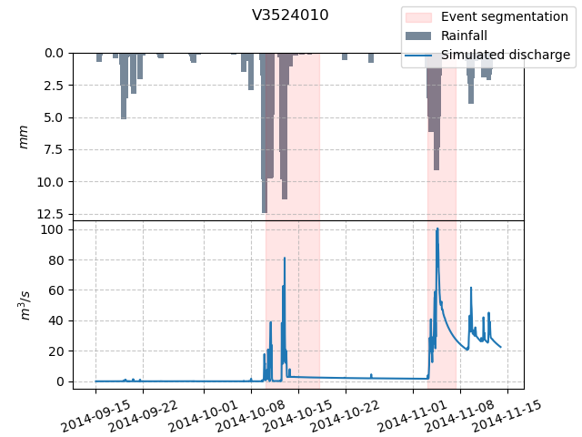
The by parameter allows us to choose whether the segmentation should be based on observed or simulated discharge data.
By default, by='obs' uses observed discharge for event segmentation. However, if we want to use simulated discharge data from a simulation for hydrograph segmentation,
we can set by='sim' to segment based on that data.
In this case, it is important to ensure that a simulation (either forward run or optimization) has been performed to generate the simulated discharge.
In [98]: model.forward_run()
</> Forward Run

In [99]: qsim = model.response.q[0, :]

In [100]: event_seg_5 = smash.hydrograph_segmentation(model, by='sim');

In [101]: event_seg_5
Out[101]:
       code               start  ...               flood  season
0  V3524010 2014-10-10 04:00:00  ... 2014-10-12 23:00:00  autumn
1  V3524010 2014-11-03 03:00:00  ... 2014-11-04 15:00:00  autumn
2  V3515010 2014-10-09 15:00:00  ... 2014-10-12 23:00:00  autumn
3  V3515010 2014-11-03 10:00:00  ... 2014-11-04 12:00:00  autumn
4  V3517010 2014-10-09 21:00:00  ... 2014-10-12 23:00:00  autumn
5  V3517010 2014-11-03 08:00:00  ... 2014-11-04 12:00:00  autumn

[6 rows x 7 columns]
Visualizing hydrograph segmented by simulated discharge of catchment V3524010:
In [102]: starts = pd.to_datetime(event_seg_5["start"])

In [103]: ends = pd.to_datetime(event_seg_5["end"])

In [104]: fig, (ax1, ax2) = plt.subplots(2, 1)

In [105]: fig.subplots_adjust(hspace=0)

In [106]: ax1.bar(dti, mean_prcp, color="lightslategrey", label="Rainfall");

In [107]: ax1.axvspan(starts[0], ends[0], alpha=.1, color="red", label="Event segmentation");

In [108]: ax1.axvspan(starts[1], ends[1], alpha=.1, color="red");

In [109]: ax1.grid(alpha=.7, ls="--")

In [110]: ax1.get_xaxis().set_visible(False)

In [111]: ax1.set_ylabel("$mm$");

In [112]: ax1.invert_yaxis()

In [113]: ax2.plot(dti, qsim, label="Simulated discharge");

In [114]: ax2.axvspan(starts[0], ends[0], alpha=.1, color="red");

In [115]: ax2.axvspan(starts[1], ends[1], alpha=.1, color="red");

In [116]: ax2.grid(alpha=.7, ls="--")

In [117]: ax2.tick_params(axis="x", labelrotation=20)

In [118]: ax2.set_ylabel("$m^3/s$");

In [119]: ax2.set_xlim(ax1.get_xlim());

In [120]: fig.legend();

In [121]: fig.suptitle("V3524010");
