Regionalization and Spatial Validation

This tutorial explains how to perform regionalization and spatial validation methods with smash using physical descriptors. The parameters \(\boldsymbol{\theta}\) can be written as a mapping \(\phi\) of descriptors \(\boldsymbol{\mathcal{D}}\) (slope, drainage density, soil water storage, etc.) and \(\boldsymbol{\rho}\), a control vector: \(\boldsymbol{\theta}(x)=\phi\left(\boldsymbol{\mathcal{D}}(x),\boldsymbol{\rho}\right)\). See the Mapping section for more details. Then the control vector of the mapping needs to be optimized: \(\boldsymbol{\hat{\rho}}=\underset{\mathrm{\boldsymbol{\rho}}}{\text{argmin}}\;J\), with \(J\) being the cost function.

We begin by opening a Python interface:

python3

Imports

We will first import the necessary libraries for this tutorial.

>>> import smash
>>> import numpy as np
>>> import pandas as pd
>>> import matplotlib.pyplot as plt

Model creation and descriptors visualization

Now, we need to create a smash.Model object. For this case, we will use the Lez dataset as an example.

Load the setup and mesh dictionaries using the smash.factory.load_dataset function and create the smash.Model object.

>>> setup, mesh = smash.factory.load_dataset("Lez")
>>> model = smash.Model(setup, mesh)

Six physical descriptors are considered in this example, which are:

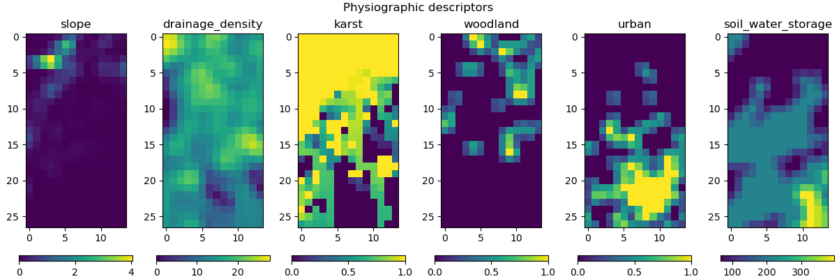
The values of these descriptors can be obtained in the physio_data derived type of the smash.Model object.

>>> model.physio_data.descriptor.shape  # (x, y, n_descriptors)

(27, 14, 6)

Note

In this tutorial, we load the setup dictionary using the smash.factory.load_dataset function. If you need to define your own setup, ensure that the keys read_descriptor, descriptor_name, and descriptor_directory are properly set.

Model simulation

Multiple linear/power mapping

Two classical approaches are commonly used for regionalization to map descriptors to parameters:

• multi-linear: a multiple linear mapping where the optimizable parameters are the coefficients.

• multi-power: a multiple power mapping where the optimizable parameters include both the coefficients and the exponents.

In this example, we use the multi-linear mapping. Before optimizing the model, it is recommended to provide a first guess for the control vector (see explanation on first guess selection for details).

>>> # First guess should be optimized for a small number of iterations
>>> optimize_options = {"termination_crit": {"maxiter": 2}}
>>> # Find first guess by optimizing the model using a uniform mapping
>>> model_ml = smash.optimize(model, optimize_options=optimize_options)

</> Optimize
    At iterate     0    nfg =     1    J = 6.85771e-01    ddx = 0.64
    At iterate     1    nfg =    30    J = 3.51670e-01    ddx = 0.64
    At iterate     2    nfg =    58    J = 1.80573e-01    ddx = 0.32
    STOP: TOTAL NO. of ITERATIONS REACHED LIMIT

Hint

You can refer to the smash.multiset_estimate() method and the Multi-set Parameters Estimate tutorial to learn how to obtain the first guess using a Bayesian-like estimate on multiple sets of solutions.

Now, we can optimize the model using the multi-linear mapping.

>>> # Optimize model using multi-linear mapping
>>> model_ml.optimize(mapping="multi-linear")

</> Optimize
    At iterate     0    nfg =     1    J = 1.80573e-01    |proj g| = 1.74191e-01
    At iterate     1    nfg =     3    J = 1.78344e-01    |proj g| = 6.51597e-02
    At iterate     2    nfg =     4    J = 1.77767e-01    |proj g| = 5.04328e-02
    At iterate     3    nfg =     5    J = 1.76513e-01    |proj g| = 3.56779e-02
    ...
    At iterate    62    nfg =    72    J = 1.31757e-01    |proj g| = 4.70840e-03
    At iterate    63    nfg =    73    J = 1.31750e-01    |proj g| = 2.37749e-03
    At iterate    64    nfg =    88    J = 1.31750e-01    |proj g| = 2.37749e-03
    CONVERGENCE: REL_REDUCTION_OF_F_<=_FACTR*EPSMCH

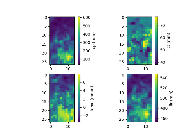
We have therefore optimized the set of rainfall-runoff parameters using a multiple linear regression constrained by physiographic descriptors. Here, most of the options used are the default ones, i.e., a minimization of one minus the Nash-Sutcliffe efficiency on the most downstream gauge of the domain. The resulting rainfall-runoff parameter maps can be viewed.

>>> f, ax = plt.subplots(2, 2)
>>>
>>> map_cp = ax[0, 0].imshow(model_ml.get_rr_parameters("cp"))
>>> f.colorbar(map_cp, ax=ax[0, 0], label="cp (mm)")
>>> map_ct = ax[0, 1].imshow(model_ml.get_rr_parameters("ct"))
>>> f.colorbar(map_ct, ax=ax[0, 1], label="ct (mm)")
>>> map_kexc = ax[1, 0].imshow(model_ml.get_rr_parameters("kexc"))
>>> f.colorbar(map_kexc, ax=ax[1, 0], label="kexc (mm/d)")
>>> map_llr = ax[1, 1].imshow(model_ml.get_rr_parameters("llr"))
>>> f.colorbar(map_llr, ax=ax[1, 1], label="llr (min)")
>>> plt.show()

The spatial validation can be performed by evaluating the model performances at non-calibrated gauges:

>>> metrics = ["NSE", "KGE"]
>>>
>>> scores = np.round(smash.evaluation(model_ml, metrics)[1:, :], 2)
>>>
>>> upstream_perf = pd.DataFrame(data=scores, index=model.mesh.code[1:], columns=metrics)
>>> upstream_perf

           NSE   KGE
Y3204030  0.80  0.63
Y3204010  0.68  0.73

Note

We used [1:] in the lists to select all the gauges except the first one, which is the downstream gauge on which the model has been calibrated.

Artificial neural network (ANN)

We can optimize the rainfall-runoff model using an ANN-based mapping of descriptors to conceptual model parameters. This is achieved by setting the mapping argument to 'ann', which is by default optimized using the Adam algorithm (see Optimization Algorithms). We can also specify several parameters for the calibration process with ANN:

• optimize_options

  • net: the neural network configuration used to learn the regionalization mapping,

  • random_state: a random seed used to initialize neural network parameters (weights and biases),

  • learning_rate: the learning rate used for weight and bias updates during training,

  • termination_crit: the maximum number of training maxiter for the neural network and a positive number to stop training when the loss function does not decrease below the current optimal value for early_stopping consecutive iterations.

• return_options

  • net: return the optimized neural network.

>>> # Get the default optimization options for ANN mapping
>>> optimize_options = smash.default_optimize_options(model, mapping="ann")
>>> optimize_options

{
    'parameters': ['cp', 'ct', 'kexc', 'llr'],
    'bounds': {'cp': (1e-06, 1000.0), 'ct': (1e-06, 1000.0), 'kexc': (-50, 50), 'llr': (1e-06, 1000.0)},
    'net':
        +---------------------------------------------------------+
        | Layer Type           Input/Output Shape  Num Parameters |
        +---------------------------------------------------------+
        | Dense                (6,)/(18,)          126            |
        | Activation (ReLU)    (18,)/(18,)         0              |
        | Dense                (18,)/(29,)         551            |
        | Activation (ReLU)    (29,)/(29,)         0              |
        | Dense                (29,)/(12,)         360            |
        | Activation (ReLU)    (12,)/(12,)         0              |
        | Dense                (12,)/(4,)          52             |
        | Activation (TanH)    (4,)/(4,)           0              |
        | Scale (MinMaxScale)  (4,)/(4,)           0              |
        +---------------------------------------------------------+
        Total parameters: 1089
        Trainable parameters: 1089,
    'learning_rate': 0.003, 'random_state': None,
    'termination_crit': {'maxiter': 200, 'early_stopping': 0}
}

In this example, we use the default neural network configuration as shown above. It indicates that the default neural network is composed of 3 hidden dense layers, each followed by a ReLU activation function. The output layer is followed by a TanH (hyperbolic tangent) function and it outputs in \(\left]-1,1\right[\) are scaled to given conceptual parameter bounds using a MinMaxScale function.

Now, we can customize several parameters such as the random state, learning rate, and early stopping criterion before optimizing the model.

>>> optimize_options["random_state"] = 0
>>> optimize_options["learning_rate"] = 0.003
>>> optimize_options["termination_crit"]["early_stopping"] = 40

>>> # Optimize model using ANN mapping
>>> model_ann, opt_ann = smash.optimize(
...     model,
...     mapping="ann",
...     optimize_options=optimize_options,
...     return_options={"net": True},
... )

</> Optimize
    At iterate     0    nfg =     1    J = 1.27958e+00    |proj g| = 1.59778e-03
    At iterate     1    nfg =     2    J = 1.26261e+00    |proj g| = 1.85001e-03
    At iterate     2    nfg =     3    J = 1.23397e+00    |proj g| = 1.41041e-03
    At iterate     3    nfg =     4    J = 1.19054e+00    |proj g| = 1.43112e-03
    ...
    At iterate   198    nfg =   199    J = 1.32467e-01    |proj g| = 7.48844e-04
    At iterate   199    nfg =   200    J = 1.32411e-01    |proj g| = 7.44386e-04
    At iterate   200    nfg =   201    J = 1.32357e-01    |proj g| = 7.40128e-04
    STOP: TOTAL NO. of ITERATIONS REACHED LIMIT

Hint

For advanced techniques, such as using customized ANNs, transfer learning, and more, refer to the in-depth tutorial on Learnable Regionalization Mapping.

The returned Optimize object opt_ann contains a Net object with the trained parameters. For example, we can access the bias of the last dense layer:

>>> opt_ann.net.get_bias()[-1]

array([[-0.18723589, -0.16801801,  0.04658873, -0.15251763]])

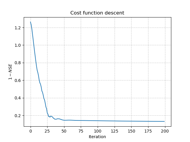
Or plot the cost function descent during the training:

>>> plt.plot(opt_ann.net.history["loss_train"])
>>> plt.xlabel("Iteration")
>>> plt.ylabel("$1-NSE$")
>>> plt.grid(alpha=.7, ls="--")
>>> plt.title("Cost function descent")
>>> plt.show()

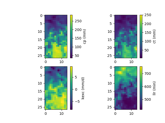
The maps of conceptual parameters optimized by the ANN mapping:

>>> f, ax = plt.subplots(2, 2)
>>>
>>> map_cp = ax[0, 0].imshow(model_ann.get_rr_parameters("cp"))
>>> f.colorbar(map_cp, ax=ax[0, 0], label="cp (mm)")
>>> map_ct = ax[0, 1].imshow(model_ann.get_rr_parameters("ct"))
>>> f.colorbar(map_ct, ax=ax[0, 1], label="ct (mm)")
>>> map_kexc = ax[1, 0].imshow(model_ann.get_rr_parameters("kexc"))
>>> f.colorbar(map_kexc, ax=ax[1, 0], label="kexc (mm/d)")
>>> map_llr = ax[1, 1].imshow(model_ann.get_rr_parameters("llr"))
>>> f.colorbar(map_llr, ax=ax[1, 1], label="llr (min)")
>>> plt.show()

Finally, we perform spatial validation on non-calibrated catchments.

>>> metrics = ["NSE", "KGE"]
>>>
>>> scores = np.round(smash.evaluation(model_ann, metrics)[1:, :], 2)
>>>
>>> upstream_perf = pd.DataFrame(data=scores, index=model.mesh.code[1:], columns=metrics)
>>> upstream_perf

           NSE   KGE
Y3204030  0.82  0.69
Y3204010  0.75  0.73