Format Description

This section describes the required format for the input data (i.e., atmospheric data, gauge information, physiographic data, and observed discharge) and their directory structure used in smash.

Input data format

Precipitation

The precipitation files must be stored for each time step of the simulation in tif format. For one time step, smash will recursively search in the prcp_directory, a file with the following name structure: *%Y%m%d%H%M*.tif (* means that we can match any character). An example of file name in tif format for the date 2014-09-15 00:00: prcp_201409150000.tif.

Note

%Y%m%d%H%M is a unique key, the prcp_directory (and all subdirectories) can not contains files with similar dates.

Potential evapotranspiration

The potential evapotranspiration files must be stored for each each time step of the simulation in tif format. For one time step, smash will recursively search in the pet_directory, a file with the following name structure: *%Y%m%d%H%M*.tif (* means that we can match any character). An example of file name in tif format for the date 2014-09-15 00:00: pet_201409150000.tif.

Note

%Y%m%d%H%M is a unique key, the pet_directory (and all subdirectories) can not contains files with similar dates.

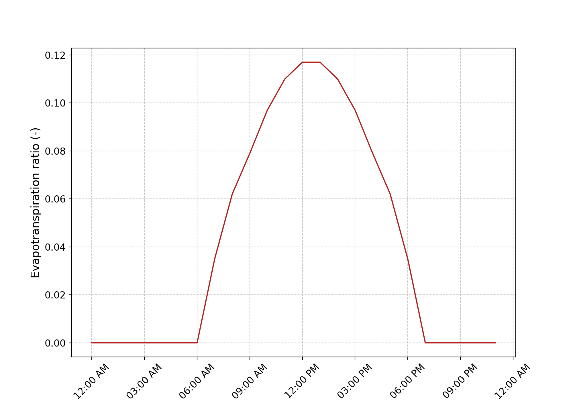
In case of daily_interannual_pet, smash will recursively search in the pet_directory, a file with the following name structure: *%m%d*.tif (* means that we can match any character). An example of file name in tif format for the day 09-15: dia_pet_0915.tif. This file will be disaggregated to the corresponding time step dt using the following distribution.

Snow

The snow files must be stored for each time step of the simulation in tif format. For one time step, smash will recursively search in the snow_directory, a file with the following name structure: *%Y%m%d%H%M*.tif (* means that we can match any character). An example of file name in tif format for the date 2014-09-15 00:00: snow_201409150000.tif.

Note

%Y%m%d%H%M is a unique key, the snow_directory (and all subdirectories) can not contains files with similar dates.

Temperature

The temperature files must be stored for each time step of the simulation in tif format. For one time step, smash will recursively search in the temp_directory, a file with the following name structure: *%Y%m%d%H%M*.tif (* means that we can match any character). An example of file name in tif format for the date 2014-09-15 00:00: temp_201409150000.tif.

Note

%Y%m%d%H%M is a unique key, the temp_directory (and all subdirectories) can not contains files with similar dates.

Gauges’ attributes

The information of the gauges can be provided by a gauge_attributes.csv file containing four columns corresponding to the code of the gauges, the spatial coordinates of outlets, and the drainage area. The spatial coordinates must be in the same unit and projection as the flow directions file (meters and Lambert 93 respectively in this example), and the drainage area in square meters.

gauge_attributes.csv

code	x	y	area
V3524010	840261	6457807	381.7
V3515010	826553	6467115	107
V3517010	828269	6469198	25.3

Physical descriptors

Physical descriptors are required for model calibration with regionalization methods. The catchment descriptors files must be stored in tif format. For each descriptor name filled in the setup argument descriptor_name, smash will recursively search in the descriptor_directory, a file with the following name structure: descriptor_name.tif. An example of file name in tif format for the slope descriptor: slope.tif.

Note

descriptor_name is a unique key, the descriptor_directory (and all subdirectories) can not contains files with similar decriptor name.

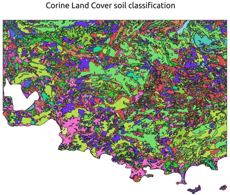
Imperviousness coefficients

The impervious proportion of a pixel’s surface is required to enhance modeling and water dynamics in the production reservoir. Imperviousness coefficients, ranging from 0 to 1, represent the percentage of a pixel’s area that is impervious to water. If not provided, the imperviousness is set to 0 by default. When using imperviousness coefficients, users must supply a tif file at the same resolution as the flow direction data. For example, the following map illustrates imperviousness based on the Corine Land Cover of the Mediterranean arc of France:

Warning

There are 4 possible warnings when reading geo-referenced data (i.e., precipitation, descriptors, etc.):

• Missing Warning

  A file (or more) is missing. It will be interpreted as no data.

• Resolution Warning

  A file (or more) has a spatial resolution different from the mesh resolution (i.e., the flow direction resolution). It will be resampled using a Nearest Neighbour algorithm.

• Overlap Warning

  A file (or more) has an origin that does not overlap with the mesh origin (i.e., the flow direction origin). The reading window is shifted towards the nearest overlapping cell.

• Out Of Bound Warning

  A file (or more) has an extent that does not include, partially or totally, the mesh extent. It will be interpreted as no data where the mesh extent is out of bound.

Observed discharge

Observed discharges are required for model calibration. The observed discharge for one catchment is read from a .csv file with the following structure:

V3524010.csv

200601010000
-99.000
-99.000
…
1.180
1.185

It is a single-column .csv file containing the observed discharge values in m³ /s (negative values in the series will be interpreted as no-data) and whose header is the first time step of the chronicle. The name of the file, for any catchment, must contains the code of the gauge which is filled in the mesh (see the smash.factory.generate_mesh method).

Note

The time step of the header does not have to match the first simulation time step. smash manages to read the corresponding lines from the setup variables, start_time, end_time and dt.

Directory structure

The aim of this section is to present the directory structure for input data and how this translates into setup.

Quick structure

Below is the most basic directory structure you can have, with one subdirectory per type of input data, and all files at the root of each subdirectory.

input_data
├── prcp
│   ├── prcp_201409150000.tif
│   ├── prcp_201409150100.tif
│   └── ...
├── pet
│   ├── pet_201409150000.tif
│   ├── pet_201409150100.tif
│   └── ...
├── snow
│   ├── snow_201409150000.tif
│   ├── snow_201409150100.tif
│   └── ...
├── temp
│   ├── temp_201409150000.tif
│   ├── temp_201409150100.tif
│   └── ...
├── qobs
│   ├── V3524010.csv
│   ├── V3504010.csv
│   └── ...
├── descriptor
│   ├── slope.tif
│   └── dd.tif
└── imperviousness
    └── imperviousness.tif

This results in the following setup:

setup = {
    "read_prcp": True,
    "prcp_directory": "./input_data/prcp",

    "read_pet": True,
    "pet_directory": "./input_data/pet",

    "read_snow": True,
    "pet_directory": "./input_data/snow",

    "read_temp": True,
    "pet_directory": "./input_data/temp",

    "read_qobs": True,
    "qobs_directory": "./input_data/qobs",

    "read_descriptor": True,
    "descriptor_directory": "./input_data/descriptor",
    "descriptor_name": ["slope", "dd"],

    "read_imperviousness": True,
    "imperviousness_file": "./input_data/imperviousness/imperviousness.tif",
}

This structure will be effective if few files are available for atmospheric data (i.e., precipitation, potential evapotranspiration, etc). However, if these directories contain a large number of files, a recursive search from the root folder can become very time-consuming. For this reason, it is necessary to adapt the directory structure to simplify and speed up file searches.

Smart structure

We can use the same type of example as above, but this time incorporate sub-directories for years, months and days in the atmospheric data.

input_data
├── prcp
│   └── 2014
│       └── 09
│           └── 15
│               ├── prcp_201409150000.tif
│               ├── prcp_201409150100.tif
│               └── ...
├── pet
│   └── 2014
│       └── 09
│           └── 15
│               ├── pet_201409150000.tif
│               ├── pet_201409150100.tif
│               └── ...
├── snow
│   └── 2014
│       └── 09
│           └── 15
│               ├── snow_201409150000.tif
│               ├── snow_201409150100.tif
│               └── ...
├── temp
│   └── 2014
│       └── 09
│           └── 15
│               ├── temp_201409150000.tif
│               ├── temp_201409150100.tif
│               └── ...
├── qobs
│   ├── V3524010.csv
│   ├── V3504010.csv
│   └── ...
├── descriptor
│   ├── slope.tif
│   └── dd.tif
└── imperviousness
    └── imperviousness.tif

At this point, the setup used previously will also work, but there will be no difference in access to files if we don’t specify directory structure. We can therefore take the previous setup and add the access method.

setup = {
    "read_prcp": True,
    "prcp_directory": "./input_data/prcp",
    "prcp_access": "%Y/%m/%d",

    "read_pet": True,
    "pet_directory": "./input_data/pet",
    "pet_access": "%Y/%m/%d",

    "read_snow": True,
    "snow_directory": "./input_data/snow",
    "snow_access": "%Y/%m/%d",

    "read_temp": True,
    "temp_directory": "./input_data/temp",
    "temp_access": "%Y/%m/%d",

    "read_qobs": True,
    "qobs_directory": "./input_data/qobs",

    "read_descriptor": True,
    "descriptor_directory": "./input_data/descriptor",
    "descriptor_name": ["slope", "dd"],

    "read_imperviousness": True,
    "imperviousness_file": "./input_data/imperviousness/imperviousness.tif",
}

The prcp_access, pet_access, snow_acces and temp_access variables should therefore be adapted to your structure to speed up data access.