Hydrological Signatures#
This section provides a detailed explanation of how to compute and visualize various hydrological signatures, which are described in the Math / Num Documentation section.
First, open a Python interface:
python3
Imports#
We will first import the necessary libraries for this tutorial.
In [1]: import smash

In [2]: import pandas as pd

In [3]: import matplotlib.pyplot as plt
Model object creation#
Now, we need to create a smash.Model object.
For this case, we will use the Cance dataset as an example.
Load the setup and mesh dictionaries using the smash.factory.load_dataset function and create the smash.Model object.
In [4]: setup, mesh = smash.factory.load_dataset("Cance")

In [5]: model = smash.Model(setup, mesh)
</> Computing mean atmospheric data
</> Adjusting GR interception capacity
Signatures computation#
We can compute the observed signatures as follows. By default, all signatures are computed, but we choose several of them.
For example, here we choose to compute the continuous runoff coefficient ('Crc'), the flow percentile at 90% ('Cfp90'),
the flood event runoff coefficient ('Erc'), and the peak flow ('Epf').
In [6]: sig_obs = smash.signatures(model, sign=["Crc", "Cfp90", "Erc", "Epf"], domain="obs")
To compute the simulated signatures, a simulation (either forward run or optimization) has to be performed to generate the simulated discharge. We compute the same signatures as the observed ones for the simulated discharge.
In [7]: model.forward_run()
</> Forward Run

In [8]: sig_sim = smash.signatures(model, sign=["Crc", "Cfp90", "Erc", "Epf"], domain="sim")
The signatures computation result object contains two attributes which are two different dictionaries:
cont: Continuous signatures computation result,event: Flood event signatures computation result.
In [9]: sig_sim.cont
Out[9]:
       code       Crc      Cfp90
0  V3524010  0.208410  27.806807
1  V3515010  0.139829   5.161739
2  V3517010  0.139431   1.355470

In [10]: sig_sim.event
Out[10]:
       code  season               start  ... multipeak       Erc         Epf
0  V3524010  autumn 2014-11-03 03:00:00  ...     False  0.322406  100.448669
1  V3515010  autumn 2014-11-03 10:00:00  ...      True  0.211647   20.168100
2  V3517010  autumn 2014-11-03 08:00:00  ...      True  0.219968    5.356512

[3 rows x 7 columns]
For flood event signatures computation, more options can be specified such as the threshold for flood event detection, the maximum duration of the flood event, etc.
The segmentation algorithm used to detect the flood events can be adjusted by setting the event_seg parameter in the smash.signatures function.
This parameter is a dictionary with keys that are the parameters used for the segmentation algorithm (refer to the tutorial on hydrograph segmentation for more details).
For instance, we can reduce the quantile threshold for flood event detection to 0.99.
In [11]: sig_obs_2 = smash.signatures(model, sign=["Erc", "Epf"], domain="obs", event_seg={"peak_quant": 0.99})

In [12]: sig_obs_2.event
Out[12]:
       code  season               start  ... multipeak       Erc         Epf
0  V3524010  autumn 2014-10-10 04:00:00  ...     False  0.566425  229.444000
1  V3524010  autumn 2014-11-03 03:00:00  ...     False  0.595655  317.380005
2  V3515010  autumn 2014-10-10 04:00:00  ...      True  0.459372   41.492001
3  V3515010  autumn 2014-11-03 10:00:00  ...      True  0.538027   49.358002
4  V3517010  autumn 2014-10-09 15:00:00  ...      True  0.403944    9.548000
5  V3517010  autumn 2014-11-03 08:00:00  ...      True  0.550013   14.939000

[6 rows x 7 columns]

In [13]: sig_sim_2 = smash.signatures(model, sign=["Erc", "Epf"], domain="sim", event_seg={"peak_quant": 0.99})

In [14]: sig_sim_2.event
Out[14]:
       code  season               start  ... multipeak       Erc         Epf
0  V3524010  autumn 2014-10-10 04:00:00  ...     False  0.070561   81.095398
1  V3524010  autumn 2014-11-03 03:00:00  ...     False  0.322406  100.448669
2  V3515010  autumn 2014-10-10 04:00:00  ...      True  0.040480   15.753152
3  V3515010  autumn 2014-11-03 10:00:00  ...      True  0.211647   20.168100
4  V3517010  autumn 2014-10-09 15:00:00  ...      True  0.031992    5.131624
5  V3517010  autumn 2014-11-03 08:00:00  ...      True  0.219968    5.356512

[6 rows x 7 columns]
Signatures visualization#
Now, we visualize, for instance, the simulated and observed peak flow in the boxplot below.
In [15]: df_obs = sig_obs_2.event

In [16]: df_sim = sig_sim_2.event

In [17]: df = pd.concat([df_obs.assign(domain="Observed"), df_sim.assign(domain="Simulated")], ignore_index=True)

In [18]: boxplot = df.boxplot(column=["Epf"], by="domain")

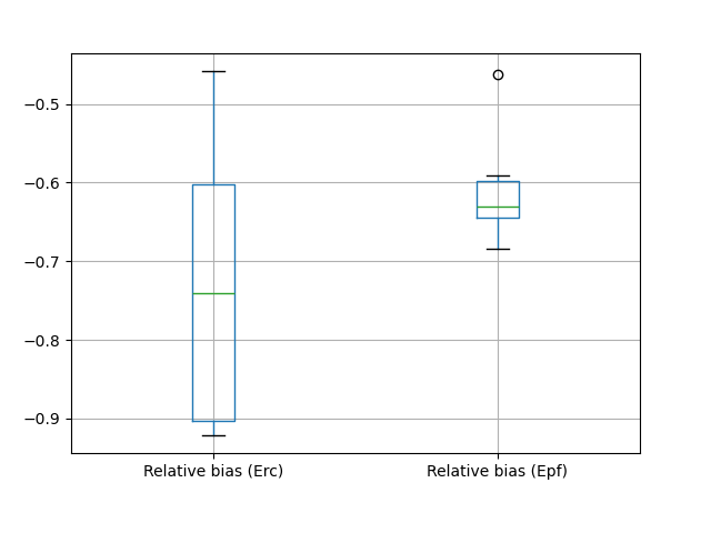
We can also compute the relative bias for any desired signature. For example, the computation and visualization of the relative bias for the two selected flood event signatures are shown below.
In [19]: ERR_Erc = sig_sim_2.event["Erc"] / sig_obs_2.event["Erc"] - 1

In [20]: ERR_Epf = sig_sim_2.event["Epf"] / sig_obs_2.event["Epf"] - 1

In [21]: df_err = pd.DataFrame({"Relative bias (Erc)": ERR_Erc, "Relative bias (Epf)": ERR_Epf})

In [22]: boxplot_err = df_err.boxplot()