Rainfall Indices#
This section aims to go into detail on how to compute and visualize precipitation indices.
First, open a Python interface:
python3
Imports#
We will first import the necessary libraries for this tutorial.
In [1]: import smash

In [2]: import numpy as np

In [3]: import matplotlib.pyplot as plt
Model object creation#
Now, we need to create a smash.Model object.
For this case, we will use the Cance dataset as an example.
Load the setup and mesh dictionaries using the smash.factory.load_dataset function and create the smash.Model object.
In [4]: setup, mesh = smash.factory.load_dataset("Cance")

In [5]: model = smash.Model(setup, mesh)
</> Computing mean atmospheric data
</> Adjusting GR interception capacity
Precipitation indices computation#
Once the smash.Model is created. The precipitation indices, computed for each gauge and each time step, are available using the smash.precipitation_indices function.
They are defined in the next section Precipitation indices description.
In [6]: res = smash.precipitation_indices(model);
The precipitation indices results are represented as a smash.PrecipitationIndices object containning 4 attributes which are 4 different indices:
std: The precipitation spatial standard deviation,d1: The first scaled moment [Zoccatelli et al., 2011],d2: The second scaled moment [Zoccatelli et al., 2011],vg: The vertical gap [Emmanuel et al., 2015] .
Each attributes (i.e. precipitation indices) of the smash.PrecipitationIndices object is a numpy.ndarray of shape (number of gauge, number of time step).
In [7]: res.std
Out[7]:
array([[nan, nan, nan, ..., nan, nan, nan],
       [nan, nan, nan, ..., nan, nan, nan],
       [nan, nan, nan, ..., nan, nan, nan]],
      shape=(3, 1440), dtype=float32)

In [8]: res.std.shape
Out[8]: (3, 1440)
Note
NaN value means that there is no precipitation at this specific gauge and time step and therefore no precipitation indices.
Precipitation indices description#
Precipitation spatial standard deviation (std)#
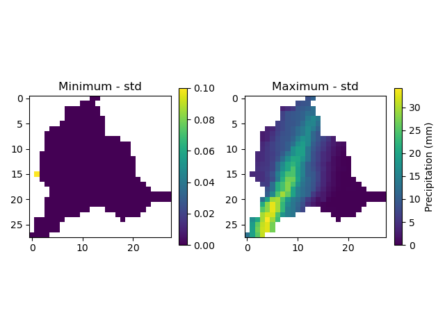
Simply the standard deviation.
Scaled moments (d1 and d2)#
The spatial scaled moments are described in Zoccatelli et al. [2011] in the section 2:
Spatial moments of catchment rainfall: definitions
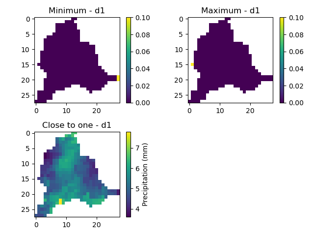
The first scaled moment \(\delta 1\) describes the distance of the centroid of catchment rainfall with respect to the average value of the flow distance (i.e. the catchment centroid). Values of \(\delta 1\) close to 1 reflect a rainfall distribution either concentrated close to the position of the catchment centroid or spatially homogeneous, with values less than one indicating that rainfall is distributed near the basin outlet, and values greater than one indicating that rainfall is distributed towards the catchment headwaters.
The second scaled moment \(\delta 2\) describes the dispersion of the rainfall-weighted flow distances about their mean value with respect to the dispersion of the flow distances. Values of \(\delta 2\) close to 1 reflect a uniform-like rainfall distribution, with values less than 1 indicating that rainfall is characterised by a unimodal distribution along the flow distance. Values greater than 1 are generally rare, and indicate cases of multimodal rainfall distributions.
Vertical gap (VG)#
The vertical gap is described in [Emmanuel et al., 2015] in the section 5.2:
The proposed indexes
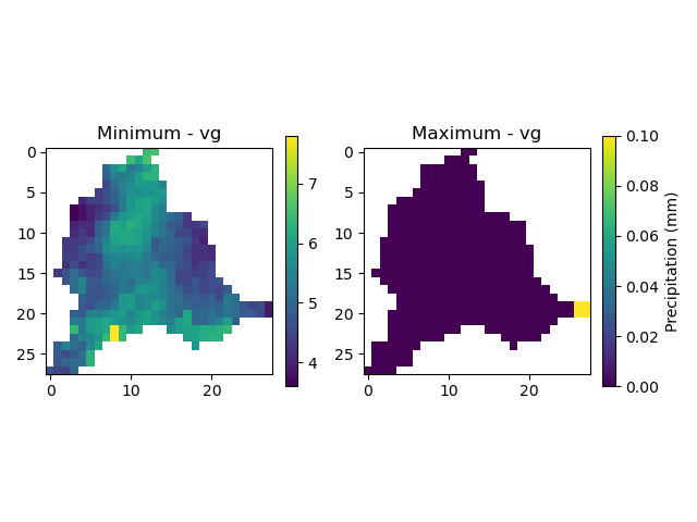
VG values close to zero indicate a rainfall distribution over the catchment revealing weak spatial variability. The higher the VG value, the more concentrated the rainfall over a small part of the catchment.
Precipitation indices visualization#
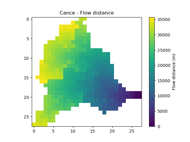
Most of the precipitation indices computations are based on flow distances. As a reminder and to facilitate the understanding of the indices values with respect to the catchment outlet and headwaters, the flow distances of the catchment are plotted below.
In [9]: flwdst = np.where(model.mesh.active_cell==0, np.nan, model.mesh.flwdst)

In [10]: plt.imshow(flwdst);

In [11]: plt.colorbar(label="Flow distance (m)");

In [12]: plt.title("Cance - Flow distance");
Let’s have nicer callable variables.
In [13]: std = res.std

In [14]: d1 = res.d1

In [15]: d2 = res.d2

In [16]: vg = res.vg

In [17]: prcp = model.atmos_data.prcp
Precipitation spatial standard deviation (std)#
Let’s start by finding out where the minimum and maximum are located for the first gauge. The methods numpy.nanargmin and numpy.nanargmax ignore NaN’s values.
In [18]: ind_min = np.nanargmin(std[0, :])

In [19]: ind_max = np.nanargmax(std[0, :])

In [20]: ind_min, ind_max
Out[20]: (np.int64(168), np.int64(666))
The associated values at those time steps are:
In [21]: std_min = std[0, ind_min]

In [22]: std_max = std[0, ind_max]

In [23]: std_min, std_max
Out[23]: (np.float32(0.0051030866), np.float32(8.763974))
We can also visualize the precipitations at those time steps, masking the non active cells.
In [24]: ma = (model.mesh.active_cell == 0)

In [25]: prcp_min = np.where(ma, np.nan, prcp[:, :, ind_min])

In [26]: prcp_max = np.where(ma, np.nan, prcp[:, :, ind_max])

In [27]: fig, ax = plt.subplots(1, 2, tight_layout=True)

In [28]: map_min = ax[0].imshow(prcp_min);

In [29]: fig.colorbar(map_min, ax=ax[0], fraction=0.05);

In [30]: ax[0].set_title("Minimum - std");

In [31]: map_max = ax[1].imshow(prcp_max);

In [32]: fig.colorbar(map_max, ax=ax[1], fraction=0.05, label="Precipitation (mm)");

In [33]: ax[1].set_title("Maximum - std");
Scaled moments (d1 and d2)#
Again we find out where the minimum and maximum are located and give the associated values.
In [34]: ind_min = np.nanargmin(d1[0, :])

In [35]: ind_max = np.nanargmax(d1[0, :])

In [36]: ind_min, ind_max
Out[36]: (np.int64(529), np.int64(168))

In [37]: d1_min = d1[0, ind_min]

In [38]: d1_max = d1[0, ind_max]

In [39]: d1_min, d1_max
Out[39]: (np.float32(0.02219003), np.float32(1.581147))
We also interested in the precipitations when the scaled moment is closed to 1.
In [40]: ind_one = np.nanargmin(np.abs(d1[0, :] - 1))

In [41]: ind_one
Out[41]: np.int64(1203)

In [42]: d1_one = d1[0, ind_one]

In [43]: d1_one
Out[43]: np.float32(1.0007353)
Then, we can visualize the precipitations at those time steps.
In [44]: ma = (model.mesh.active_cell == 0)

In [45]: prcp_min = np.where(ma, np.nan, prcp[:, :, ind_min])

In [46]: prcp_max = np.where(ma, np.nan, prcp[:, :, ind_max])

In [47]: prcp_one = np.where(ma, np.nan, prcp[:, :, ind_one])

In [48]: fig, ax = plt.subplots(2, 2, tight_layout=True)

In [49]: map_min = ax[0, 0].imshow(prcp_min);

In [50]: fig.colorbar(map_min, ax=ax[0, 0]);

In [51]: ax[0, 0].set_title("Minimum - d1");

In [52]: map_max = ax[0, 1].imshow(prcp_max);

In [53]: fig.colorbar(map_max, ax=ax[0, 1]);

In [54]: ax[0, 1].set_title("Maximum - d1");

In [55]: map_one = ax[1, 0].imshow(prcp_one);

In [56]: fig.colorbar(map_one, ax=ax[1, 0], label="Precipitation (mm)");

In [57]: ax[1, 0].set_title("Close to one - d1");

In [58]: ax[1, 1].axis('off');
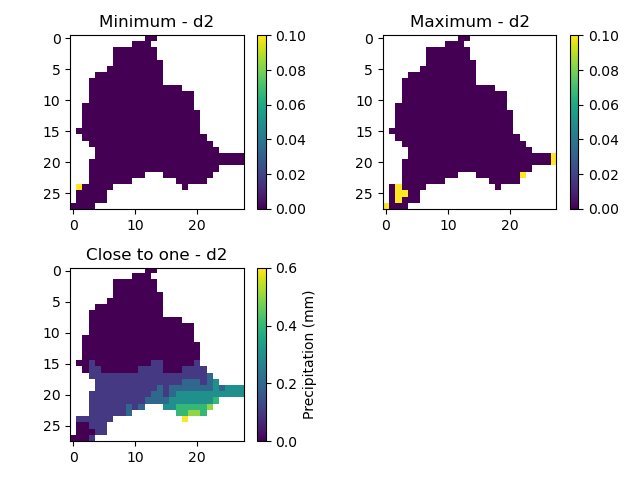
Applying the same principle to the d2 moment:
In [59]: ind_min = np.nanargmin(d2[0, :])

In [60]: ind_max = np.nanargmax(d2[0, :])

In [61]: ind_one = np.nanargmin(np.abs(d2[0, :] - 1))

In [62]: ind_min, ind_max, ind_one
Out[62]: (np.int64(648), np.int64(633), np.int64(527))

In [63]: d2_min = d2[0, ind_min]

In [64]: d2_max = d2[0, ind_max]

In [65]: d2_one = d2[0, ind_one]

In [66]: d2_min, d2_max, d2_one
Out[66]: (np.float32(1.6027067e-07), np.float32(2.9966123), np.float32(0.9987884))

In [67]: ma = (model.mesh.active_cell == 0)

In [68]: prcp_min = np.where(ma, np.nan, prcp[:, :, ind_min])

In [69]: prcp_max = np.where(ma, np.nan, prcp[:, :, ind_max])

In [70]: prcp_one = np.where(ma, np.nan, prcp[:, :, ind_one])

In [71]: f, ax = plt.subplots(2, 2, tight_layout=True)

In [72]: map_min = ax[0, 0].imshow(prcp_min);

In [73]: f.colorbar(map_min, ax=ax[0, 0]);

In [74]: ax[0, 0].set_title("Minimum - d2");

In [75]: map_max = ax[0, 1].imshow(prcp_max);

In [76]: f.colorbar(map_max, ax=ax[0, 1]);

In [77]: ax[0, 1].set_title("Maximum - d2");

In [78]: map_one = ax[1, 0].imshow(prcp_one);

In [79]: f.colorbar(map_one, ax=ax[1, 0], label="Precipitation (mm)");

In [80]: ax[1, 0].set_title("Close to one - d2");

In [81]: ax[1, 1].axis('off');
Vertical gap (VG)#
Finally, applying the same principle to the vertical gap:
In [82]: ind_min = np.nanargmin(vg[0, :])

In [83]: ind_max = np.nanargmax(vg[0, :])

In [84]: ind_min, ind_max
Out[84]: (np.int64(1203), np.int64(234))

In [85]: vg_min = res.vg[0, ind_min]

In [86]: vg_max = res.vg[0, ind_max]

In [87]: vg_min, vg_max
Out[87]: (np.float32(0.014617026), np.float32(0.98433423))

In [88]: ma = (model.mesh.active_cell == 0)

In [89]: prcp_min = np.where(ma, np.nan, prcp[:,:,ind_min])

In [90]: prcp_max = np.where(ma, np.nan, prcp[:,:,ind_max])

In [91]: fig, ax = plt.subplots(1, 2, tight_layout=True)

In [92]: map_min = ax[0].imshow(prcp_min);

In [93]: fig.colorbar(map_min, ax=ax[0], fraction=0.05);

In [94]: ax[0].set_title("Minimum - vg");

In [95]: map_max = ax[1].imshow(prcp_max);

In [96]: fig.colorbar(map_max, ax=ax[1], fraction=0.05, label="Precipitation (mm)");

In [97]: ax[1].set_title("Maximum - vg");