Large Domain Simulation

This tutorial aims to perform a simulation over the whole of metropolitan France with a simple model structure. The objective is to create a mesh over a large spatial domain, to perform a forward run and to visualize the simulated discharge over the entire domain. We begin by opening a Python interface:

python3

Imports

We will first import the necessary libraries for this tutorial. Both LogNorm and SymLogNorm will be used for plotting.

In [1]: import smash

In [2]: import numpy as np

In [3]: import matplotlib.pyplot as plt

In [4]: from matplotlib.colors import LogNorm, SymLogNorm

Model creation

Now, we need to create a smash.Model object. For this case, we will use the France dataset as an example.

Load the setup and mesh dictionaries using the smash.factory.load_dataset function and create the smash.Model object.

In [5]: setup, mesh = smash.factory.load_dataset("France")

In [6]: model = smash.Model(setup, mesh)
</> Computing mean atmospheric data
</> Adjusting GR interception capacity

Model simulation with a forward run

We can now call the Model.forward_run method, but by default and for memory reasons, the simulated discharge on the entire spatio-temporal domain is not saved. This means storing an numpy.ndarray of shape (nrow, ncol, ntime_step), which may be quite large depending on the simulation period and the spatial domain. To activate this option, the return_options argument must be filled in, specifying that you want to retrieve the simulated discharge on the whole domain. Whenever the return_options is filled in, the Model.forward_run method returns a smash.ForwardRun object storing these variables.

In [7]: fwd_run = model.forward_run(return_options={"q_domain": True})

In [8]: fwd_run
Out[8]: 
  q_domain: <class 'numpy.ndarray'>
 time_step: <class 'pandas.core.indexes.datetimes.DatetimeIndex'>

In [9]: fwd_run.time_step
Out[9]: 
DatetimeIndex(['2012-01-01 01:00:00', '2012-01-01 02:00:00',
               '2012-01-01 03:00:00', '2012-01-01 04:00:00',
               '2012-01-01 05:00:00', '2012-01-01 06:00:00',
               '2012-01-01 07:00:00', '2012-01-01 08:00:00',
               '2012-01-01 09:00:00', '2012-01-01 10:00:00',
               '2012-01-01 11:00:00', '2012-01-01 12:00:00',
               '2012-01-01 13:00:00', '2012-01-01 14:00:00',
               '2012-01-01 15:00:00', '2012-01-01 16:00:00',
               '2012-01-01 17:00:00', '2012-01-01 18:00:00',
               '2012-01-01 19:00:00', '2012-01-01 20:00:00',
               '2012-01-01 21:00:00', '2012-01-01 22:00:00',
               '2012-01-01 23:00:00', '2012-01-02 00:00:00',
               '2012-01-02 01:00:00', '2012-01-02 02:00:00',
               '2012-01-02 03:00:00', '2012-01-02 04:00:00',
               '2012-01-02 05:00:00', '2012-01-02 06:00:00',
               '2012-01-02 07:00:00', '2012-01-02 08:00:00'],
              dtype='datetime64[ns]', freq='3600s')

In [10]: fwd_run.q_domain.shape
Out[10]: (1075, 1150, 32)

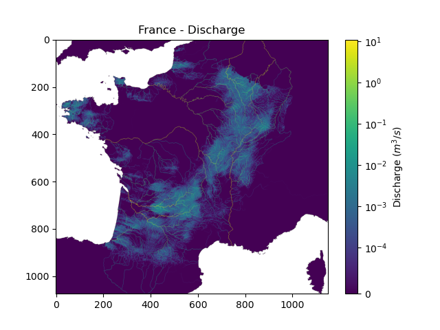
The returned object smash.ForwardRun contains two variables q_domain and time_step. With q_domain a numpy.ndarray of shape (nrow, ncol, ntime_step) storing the simulated discharge and time_step a pandas.DatetimeIndex storing the saved time steps. We can view the simulated discharge for one time step, for example the last one.

In [11]: q = fwd_run.q_domain[..., -1]

In [12]: q = np.where(model.mesh.active_cell == 0, np.nan, q) # Remove the non-active cells from the plot

In [13]: plt.imshow(q, norm=SymLogNorm(1e-4));

In [14]: plt.colorbar(label="Discharge $(m^3/s)$");

In [15]: plt.title("France - Discharge");

Note

Given that we performed a forward run on only 32 time steps with default rainfall-runoff parameters and initial states, the simulated discharge is not realistic.

By default, if the returned time steps are not defined, all the time steps are returned. It is possible to return only certain time steps by specifying them in the return_options argument, for example only the two last ones.

In [16]: time_step = ["2012-01-02 07:00", "2012-01-02 08:00"]  # define returned time steps

In [17]: fwd_run = model.forward_run(
   ....:     return_options={
   ....:         "time_step": time_step,
   ....:         "q_domain": True
   ....:     }
   ....: )  # forward run and return q_domain at specified time steps
   ....: 

In [18]: fwd_run.time_step
Out[18]: DatetimeIndex(['2012-01-02 07:00:00', '2012-01-02 08:00:00'], dtype='datetime64[ns]', freq=None)

In [19]: fwd_run.q_domain.shape
Out[19]: (1075, 1150, 2)

In [20]: q = fwd_run.q_domain[..., -1]

In [21]: q = np.where(model.mesh.active_cell == 0, np.nan, q) # Remove the non-active cells from the plot

In [22]: plt.imshow(q, norm=SymLogNorm(1e-4));

In [23]: plt.colorbar(label="Discharge $(m^3/s)$");

In [24]: plt.title("France - Discharge");