Model Object Initialization

smash methods are constructed around a Model object. This section details how to initialize this Model object and provides descriptions of the Model attributes. The tutorial uses data downloaded from the Cance dataset section.

Let’s start by opening a Python interface. For this tutorial, assume that the example dataset has been downloaded and is located at the following path: './Cance-dataset/'.

python3

Imports

We will first import the necessary libraries for this tutorial.

In [1]: import smash

In [2]: import pandas as pd

In [3]: import matplotlib.pyplot as plt

Hint

The visualization library matplotlib is not installed by default but can be installed with pip as follows:

pip install matplotlib

Setup creation

To create the smash.Model object, we need to define the setup and the mesh. See the tutorial on Hydrological Mesh Construction for mesh generation.

The setup is a Python dictionary (i.e., pairs of keys and values) which contains all information relating to the simulation period, the structure of the hydrological model and the reading of input data. For this first simulation let us create the following setup:

In [4]: setup = {
   ...:     "start_time": "2014-09-15 00:00",
   ...:     "end_time": "2014-11-14 00:00",
   ...:     "dt": 3_600,
   ...:     "hydrological_module": "gr4",
   ...:     "routing_module": "lr",
   ...:     "read_qobs": True,
   ...:     "qobs_directory": "./Cance-dataset/qobs",
   ...:     "read_prcp": True,
   ...:     "prcp_conversion_factor": 0.1,
   ...:     "prcp_directory": "./Cance-dataset/prcp",
   ...:     "read_pet": True,
   ...:     "daily_interannual_pet": True,
   ...:     "pet_directory": "./Cance-dataset/pet",
   ...: }
   ...: 

To get into more details, this setup is composed of:

• start_time

  The beginning of the simulation,

• end_time

  The end of the simulation,

• dt

  The simulation time step in second,

Note

The convention of smash is that start_time is the date used to initialize the model’s states. All the modeled state-flux variables (i.e., discharge, states, internal fluxes) will be computed over the period start_time + 1dt and end_time

• hydrological_module

  The hydrological module could be for instance gr4, gr5, grd, loieau or vic3l.

  Hint

  See the Hydrological Module section

• routing_module

  The routing module, to be chosen from [lag0, lr, kw],

  Hint

  See the Routing Module section

• read_qobs

  Whether or not to read observed discharges files,

• qobs_directory

  The path to the observed discharges files,

• read_prcp

  Whether or not to read precipitation files,

• prcp_conversion_factor

  The precipitation conversion factor (the precipitation value in data, for example in \(1/10 mm\), will be multiplied by the conversion factor to reach precipitation in \(mm\) as needed by the hydrological modules),

• prcp_directory

  The path to the precipitation files,

• read_pet

  Whether or not to read potential evapotranspiration files,

• pet_conversion_factor

  The potential evapotranspiration conversion factor (the potential evapotranspiration value from data will be multiplied by the conversion factor to get \(mm\) as needed by the hydrological modules),

• daily_interannual_pet

  Whether or not to read potential evapotranspiration files as daily interannual value desaggregated to the corresponding time step dt,

• pet_directory

  The path to the potential evapotranspiration files,

In summary the current setup you defined above corresponds to :

• a simulation time window between 2014-09-15 00:00 and 2014-11-14 00:00 at an hourly time step.

• a hydrological model structure composed of the hydrological module gr4 applied on each pixel of the mesh and coupled to the routing module lr (linear reservoir) for conveying discharge from pixels to pixel downstream.

• input data of observed discharge, precipitation and potential evapotranspiration will be read from the directories defined in the setup and containing the previously downloaded case data. A few options have been added for some of the input data, the conversion factor for precipitation, given that our data is in tenths of a millimeter, and the information that we want to work with daily interannual potential evapotranspiration data.

Hint

Detailed information on the model setup can be obtained from the API reference section of smash.Model.

Save the setup

To avoid regenerating the setup for each simulation with the same case study, we can save it using the smash.io.save_setup function. This function stores the setup under YAML format, which can later be read back using the smash.io.read_setup function.

In [5]: smash.io.save_setup(setup, "setup.yaml")

In [6]: setup = smash.io.read_setup("setup.yaml")

In [7]: setup.keys()
Out[7]: dict_keys(['daily_interannual_pet', 'dt', 'end_time', 'hydrological_module', 'pet_directory', 'prcp_conversion_factor', 'prcp_directory', 'qobs_directory', 'read_pet', 'read_prcp', 'read_qobs', 'routing_module', 'start_time'])

Hint

The setups of demo data in smash can also be loaded using the function smash.factory.load_dataset.

Model initialization and attributes

Note that the tutorial on mesh generation has been detailed previously. In this guide, we use smash.factory.load_dataset to load a demo mesh instead of recreating it for simplicity.

In [8]: _, mesh = smash.factory.load_dataset("Cance")

Initialize the Model object by passing the setup and the mesh to the smash.Model constructor.

In [9]: model = smash.Model(setup, mesh)
</> Computing mean atmospheric data
</> Adjusting GR interception capacity

In [10]: model
Out[10]: 
Model
    atmos_data: ['mean_pet', 'mean_prcp', '...', 'sparse_prcp', 'sparse_snow']
    mesh: ['active_cell', 'area', '...', 'xres', 'ymax']
    nn_parameters: ['bias_1', 'bias_2', '...', 'weight_1', 'weight_2']
    physio_data: ['descriptor', 'imperviousness', 'l_descriptor', 'u_descriptor']
    response: ['q']
    response_data: ['q']
    rr_final_states: ['keys', 'values']
    rr_initial_states: ['keys', 'values']
    rr_parameters: ['keys', 'values']
    serr_mu_parameters: ['keys', 'values']
    serr_sigma_parameters: ['keys', 'values']
    setup: ['adjust_interception', 'compute_mean_atmos', '...', 'temp_access', 'temp_directory']
    u_response_data: ['q_stdev']

The smash.Model object is a complex structure with several attributes and associated methods. Not all of these will be detailed in this tutorial. As you can see by displaying the smash.Model object above after initializing it, several attributes are accessible:

Setup

Model.setup contains all the information previously passed through the setup dictionary plus a set of other variables filled in by default or potentially not used afterwards.

In [11]: model.setup.start_time, model.setup.end_time, model.setup.dt
Out[11]: ('2014-09-15 00:00', '2014-11-14 00:00', 3600.0)

Mesh

Model.mesh contains all the information previously passed through the mesh dictionary.

In [12]: model.mesh.nrow, model.mesh.ncol, model.mesh.nac
Out[12]: (28, 28, 383)

In [13]: plt.imshow(model.mesh.flwdir);

In [14]: plt.colorbar(label="Flow direction (D8)");

In [15]: plt.title("Cance - Flow direction");

Note

Once the smash.Model object is initialized, the numpy.ndarray of the mesh are not masked anymore in the Model.mesh. It is therefore normal to have a difference in the non-active cells.

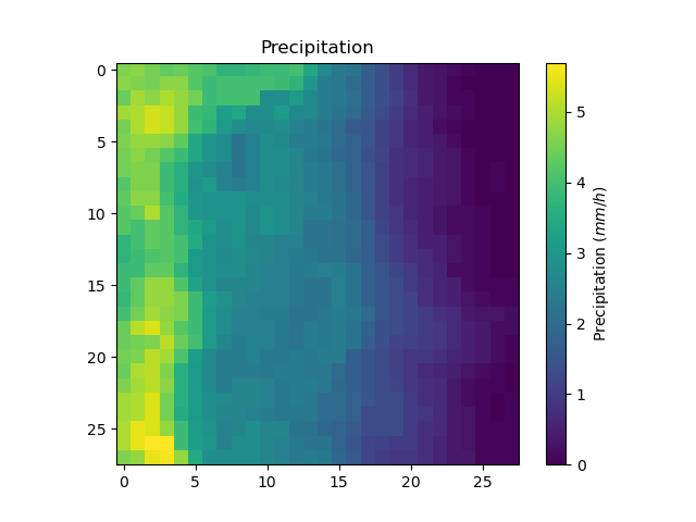
Atmospheric data

Model.atmos_data contains all the atmospheric data, here precipitation (prcp) and potential evapotranspiration (pet) that are stored as numpy.ndarray of shape (nrow, ncol, ntime_step) (one 2D array per time step). We can visualize the value of precipitation for an arbitrary time step.

In [16]: plt.imshow(model.atmos_data.prcp[..., 1200]);

In [17]: plt.colorbar(label="Precipitation ($mm/h$)");

In [18]: plt.title("Precipitation");

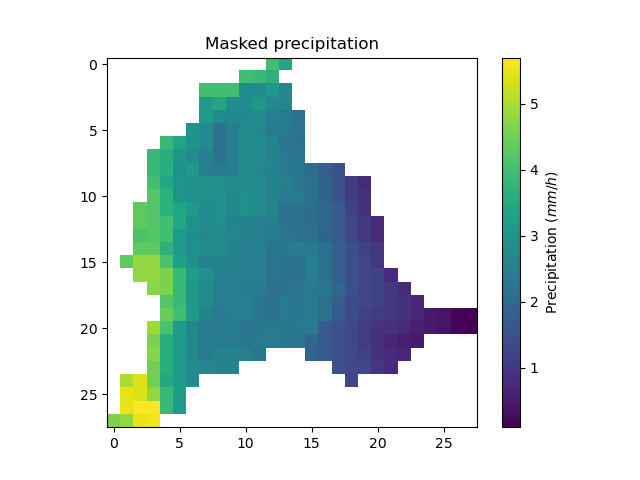
Or masked on the active cells of the catchment

In [19]: ma_prcp = np.where(
   ....:     model.mesh.active_cell == 0,
   ....:     np.nan,
   ....:     model.atmos_data.prcp[..., 1200]
   ....: )
   ....: 

In [20]: plt.imshow(ma_prcp);

In [21]: plt.colorbar(label="Precipitation ($mm/h$)");

In [22]: plt.title("Masked precipitation");

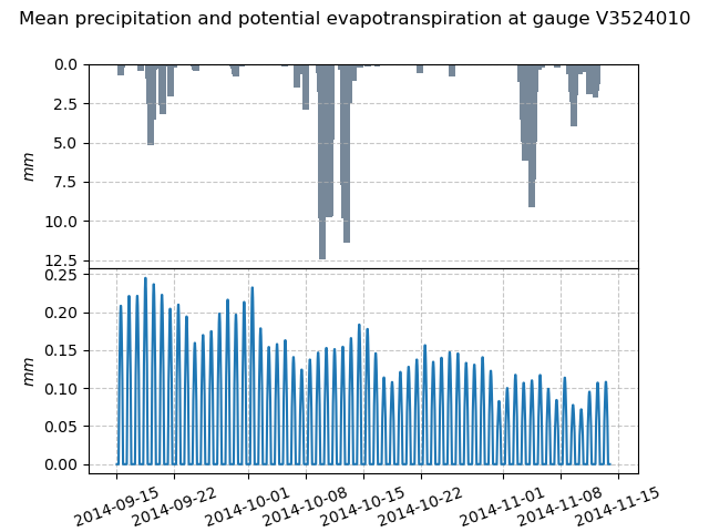
The spatial average of precipitation (mean_prcp) and potential evapotranspiration (mean_pet) over each gauge are also computed and stored in Model.atmos_data. They are numpy.ndarray of shape (ng, ntime_step), one temporal series by gauge.

In [23]: dti = pd.date_range(start=model.setup.start_time, end=model.setup.end_time, freq="h")[1:]

In [24]: mean_pet = model.atmos_data.mean_pet[0, :]

In [25]: mean_prcp = model.atmos_data.mean_prcp[0, :]

In [26]: code = model.mesh.code[0]

In [27]: fig, (ax1, ax2) = plt.subplots(2, 1)

In [28]: fig.subplots_adjust(hspace=0)

In [29]: ax1.bar(dti, mean_prcp, color="lightslategrey", label="Rainfall");

In [30]: ax1.grid(alpha=.7, ls="--")

In [31]: ax1.get_xaxis().set_visible(False)

In [32]: ax1.set_ylabel("$mm$");

In [33]: ax1.invert_yaxis()

In [34]: ax2.plot(dti, mean_pet, label="Evapotranspiration");

In [35]: ax2.grid(alpha=.7, ls="--")

In [36]: ax2.tick_params(axis="x", labelrotation=20)

In [37]: ax2.set_ylabel("$mm$");

In [38]: ax2.set_xlim(ax1.get_xlim());

In [39]: fig.suptitle(
   ....:     f"Mean precipitation and potential evapotranspiration at gauge {code}"
   ....: );
   ....: 

Response data

Model.response_data contains all the model response data. Currently, the only model response data is the observed discharge (q). The observed discharge is a numpy.ndarray of shape (ng, ntime_step), one temporal series by gauge.

In [40]: code = model.mesh.code[0]

In [41]: plt.plot(model.response_data.q[0, :]);

In [42]: plt.grid(ls="--", alpha=.7);

In [43]: plt.xlabel("Time step");

In [44]: plt.ylabel("Discharge ($m^3/s$)")
Out[44]: Text(0, 0.5, 'Discharge ($m^3/s$)')

In [45]: plt.title(
   ....:     f"Observed discharge at gauge {code}"
   ....: );
   ....: 

Rainfall-runoff parameters

Model.rr_parameters contains all the rainfall-runoff parameters. The rainfall-runoff parameters available depend on the chosen model structure and of the different modules that compose it. Here, we have selected the hydrological module gr4 and the routing module lr. This attribute consists of one variable storing the keys i.e., the names of the rainfall-runoff parameters and another storing their values, a numpy.ndarray of shape (nrow, ncol, nrrp), where nrrp is the number of rainfall-runoff parameters available.

In [46]: model.setup.nrrp, model.rr_parameters.keys
Out[46]: (5, array(['ci', 'cp', 'ct', 'kexc', 'llr'], dtype='<U128'))

To access the values of a specific rainfall-runoff parameter, it is possible to use the Model.get_rr_parameters method, here applied to get the spatial values of the production reservoir capacity

In [47]: model.get_rr_parameters("cp")[:10, :10] # Avoid printing all the cells
Out[47]: 
array([[200., 200., 200., 200., 200., 200., 200., 200., 200., 200.],
       [200., 200., 200., 200., 200., 200., 200., 200., 200., 200.],
       [200., 200., 200., 200., 200., 200., 200., 200., 200., 200.],
       [200., 200., 200., 200., 200., 200., 200., 200., 200., 200.],
       [200., 200., 200., 200., 200., 200., 200., 200., 200., 200.],
       [200., 200., 200., 200., 200., 200., 200., 200., 200., 200.],
       [200., 200., 200., 200., 200., 200., 200., 200., 200., 200.],
       [200., 200., 200., 200., 200., 200., 200., 200., 200., 200.],
       [200., 200., 200., 200., 200., 200., 200., 200., 200., 200.],
       [200., 200., 200., 200., 200., 200., 200., 200., 200., 200.]],
      dtype=float32)

The rainfall-runoff parameters are filled in with default spatially uniform values but can be modified using the Model.set_rr_parameters

In [48]: model.set_rr_parameters("cp", 134)

In [49]: model.get_rr_parameters("cp")[:10, :10]
Out[49]: 
array([[134., 134., 134., 134., 134., 134., 134., 134., 134., 134.],
       [134., 134., 134., 134., 134., 134., 134., 134., 134., 134.],
       [134., 134., 134., 134., 134., 134., 134., 134., 134., 134.],
       [134., 134., 134., 134., 134., 134., 134., 134., 134., 134.],
       [134., 134., 134., 134., 134., 134., 134., 134., 134., 134.],
       [134., 134., 134., 134., 134., 134., 134., 134., 134., 134.],
       [134., 134., 134., 134., 134., 134., 134., 134., 134., 134.],
       [134., 134., 134., 134., 134., 134., 134., 134., 134., 134.],
       [134., 134., 134., 134., 134., 134., 134., 134., 134., 134.],
       [134., 134., 134., 134., 134., 134., 134., 134., 134., 134.]],
      dtype=float32)

In [50]: model.set_rr_parameters("cp", 200) # Set the default value back

Rainfall-runoff initial states

Model.rr_initial_states contains all the rainfall-runoff initial states. This attribute is very similar to the rainfall-runoff parameters, both in its construction and in the variables it contains.

In [51]: model.setup.nrrs, model.rr_initial_states.keys
Out[51]: (4, array(['hi', 'hp', 'ht', 'hlr'], dtype='<U128'))

Methods similar to those used for rainfall-runoff parameters are available for states

In [52]: model.get_rr_initial_states("hp")[:10, :10]
Out[52]: 
array([[0.01, 0.01, 0.01, 0.01, 0.01, 0.01, 0.01, 0.01, 0.01, 0.01],
       [0.01, 0.01, 0.01, 0.01, 0.01, 0.01, 0.01, 0.01, 0.01, 0.01],
       [0.01, 0.01, 0.01, 0.01, 0.01, 0.01, 0.01, 0.01, 0.01, 0.01],
       [0.01, 0.01, 0.01, 0.01, 0.01, 0.01, 0.01, 0.01, 0.01, 0.01],
       [0.01, 0.01, 0.01, 0.01, 0.01, 0.01, 0.01, 0.01, 0.01, 0.01],
       [0.01, 0.01, 0.01, 0.01, 0.01, 0.01, 0.01, 0.01, 0.01, 0.01],
       [0.01, 0.01, 0.01, 0.01, 0.01, 0.01, 0.01, 0.01, 0.01, 0.01],
       [0.01, 0.01, 0.01, 0.01, 0.01, 0.01, 0.01, 0.01, 0.01, 0.01],
       [0.01, 0.01, 0.01, 0.01, 0.01, 0.01, 0.01, 0.01, 0.01, 0.01],
       [0.01, 0.01, 0.01, 0.01, 0.01, 0.01, 0.01, 0.01, 0.01, 0.01]],
      dtype=float32)

In [53]: model.set_rr_initial_states("hp", 0.23)

In [54]: model.get_rr_initial_states("hp")[:10, :10]
Out[54]: 
array([[0.23, 0.23, 0.23, 0.23, 0.23, 0.23, 0.23, 0.23, 0.23, 0.23],
       [0.23, 0.23, 0.23, 0.23, 0.23, 0.23, 0.23, 0.23, 0.23, 0.23],
       [0.23, 0.23, 0.23, 0.23, 0.23, 0.23, 0.23, 0.23, 0.23, 0.23],
       [0.23, 0.23, 0.23, 0.23, 0.23, 0.23, 0.23, 0.23, 0.23, 0.23],
       [0.23, 0.23, 0.23, 0.23, 0.23, 0.23, 0.23, 0.23, 0.23, 0.23],
       [0.23, 0.23, 0.23, 0.23, 0.23, 0.23, 0.23, 0.23, 0.23, 0.23],
       [0.23, 0.23, 0.23, 0.23, 0.23, 0.23, 0.23, 0.23, 0.23, 0.23],
       [0.23, 0.23, 0.23, 0.23, 0.23, 0.23, 0.23, 0.23, 0.23, 0.23],
       [0.23, 0.23, 0.23, 0.23, 0.23, 0.23, 0.23, 0.23, 0.23, 0.23],
       [0.23, 0.23, 0.23, 0.23, 0.23, 0.23, 0.23, 0.23, 0.23, 0.23]],
      dtype=float32)

In [55]: model.set_rr_initial_states("hp", 0.01) # Set the default value back

Rainfall-runoff final states

Model.rr_final_states contains all the rainfall-runoff final states, i.e., at the end of the simulation time window defined in setup. This attribute is identical to the rainfall-runoff initial states but for final ones. The final states are updated once a simulation is performed.

In [56]: model.setup.nrrs, model.rr_final_states.keys
Out[56]: (4, array(['hi', 'hp', 'ht', 'hlr'], dtype='<U128'))

Rainfall-runoff final states only have getters and are by default filled in with -99 until a simulation has been performed.

In [57]: model.get_rr_final_states("hp")[:10, :10]
Out[57]: 
array([[-99., -99., -99., -99., -99., -99., -99., -99., -99., -99.],
       [-99., -99., -99., -99., -99., -99., -99., -99., -99., -99.],
       [-99., -99., -99., -99., -99., -99., -99., -99., -99., -99.],
       [-99., -99., -99., -99., -99., -99., -99., -99., -99., -99.],
       [-99., -99., -99., -99., -99., -99., -99., -99., -99., -99.],
       [-99., -99., -99., -99., -99., -99., -99., -99., -99., -99.],
       [-99., -99., -99., -99., -99., -99., -99., -99., -99., -99.],
       [-99., -99., -99., -99., -99., -99., -99., -99., -99., -99.],
       [-99., -99., -99., -99., -99., -99., -99., -99., -99., -99.],
       [-99., -99., -99., -99., -99., -99., -99., -99., -99., -99.]],
      dtype=float32)

Response

Model.response contains all the model response. Similar to the model response data, the only model response is the discharge (q). The discharge is a numpy.ndarray of shape (ng, ntime_step), one temporal series by gauge.

In [58]: model.response.q
Out[58]: 
array([[-99., -99., -99., ..., -99., -99., -99.],
       [-99., -99., -99., ..., -99., -99., -99.],
       [-99., -99., -99., ..., -99., -99., -99.]],
      shape=(3, 1440), dtype=float32)

Similar to rainfall-runoff final states, the response discharge is updated each time a simulation is performed. At initialization, response discharge is filled in with -99.