Hydrological Mesh Construction

This section explains the hydrological mesh construction and details how to generate and visualize this mesh. The tutorial uses data downloaded from the Cance dataset section.

Let’s start by opening a Python interface. For this tutorial, assume that the example dataset has been downloaded and is located at the following path: './Cance-dataset/'.

python3

Imports

Let’s begin by importing the necessary libraries for this tutorial.

In [1]: import smash

In [2]: import pandas as pd

In [3]: import matplotlib.pyplot as plt

Hint

The visualization library matplotlib is not installed by default but can be installed with pip as follows:

pip install matplotlib

Mesh construction

The mesh is a Python dictionary generated using the smash.factory.generate_mesh function. This function requires a flow direction file France_flwdir.tif and gauge attributes information from gauge_attributes.csv (see the Gauges’ attributes section in Format Description).

In [4]: gauge_attributes = pd.read_csv("./Cance-dataset/gauge_attributes.csv")

In [5]: mesh = smash.factory.generate_mesh(
   ...:     flwdir_path="./Cance-dataset/France_flwdir.tif",
   ...:     x=list(gauge_attributes["x"]),
   ...:     y=list(gauge_attributes["y"]),
   ...:     area=list(gauge_attributes["area"] * 1e6), # Convert km² to m²
   ...:     code=list(gauge_attributes["code"]),
   ...: )
   ...: 

In [6]: mesh.keys()
Out[6]: dict_keys(['xres', 'yres', 'xmin', 'ymax', 'nrow', 'ncol', 'dx', 'dy', 'flwdir', 'flwdst', 'flwacc', 'npar', 'ncpar', 'cscpar', 'cpar_to_rowcol', 'flwpar', 'nac', 'active_cell', 'ng', 'gauge_pos', 'code', 'area', 'area_dln'])

Note

By default, the bounding box—i.e., the extent of the domain—is automatically computed as the smallest possible rectangle that encloses the boundaries of the hydrological catchments. However, users can specify a custom bounding box if desired. The bounding box is defined as a list of four coordinate values: bbox = [xmin, xmax, ymin, ymax], where x refers to latitude and y to longitude.

In [7]: mesh = smash.factory.generate_mesh(
   ...:     flwdir_path="./Cance-dataset/France_flwdir.tif",
   ...:     bbox=[800000.,  850000., 6440000., 6490000.],
   ...:     x=list(gauge_attributes["x"]),
   ...:     y=list(gauge_attributes["y"]),
   ...:     area=list(gauge_attributes["area"] * 1e6), # Convert km² to m²
   ...:     code=list(gauge_attributes["code"]),
   ...: )
   ...: 

If the specified bounding box is smaller than the extent of the hydrological catchments, the corresponding outlets will be excluded from the mesh, and a warning message will be returned.

The gauge attributes can also be passed directly without using a csv file.

In [8]: mesh = smash.factory.generate_mesh(
   ...:     flwdir_path="./Cance-dataset/France_flwdir.tif",
   ...:     x=[840_261, 826_553, 828_269],
   ...:     y=[6_457_807, 6_467_115, 6_469_198],
   ...:     area=[381.7 * 1e6, 107 * 1e6, 25.3 * 1e6], # Convert km² to m²
   ...:     code=["V3524010", "V3515010", "V3517010"],
   ...: )
   ...: 

Mesh attributes and visualization

To get into more details, this mesh is composed of:

• xres, yres

  The spatial resolution (unit of the flow directions map, meter)

  In [9]: mesh["xres"], mesh["yres"]
  Out[9]: (1000.0, 1000.0)
  

• xmin, ymax

  The coordinates of the upper left corner (unit of the flow directions map, meter)

  In [10]: mesh["xmin"], mesh["ymax"]
  Out[10]: (np.float64(813000.0), np.float64(6478000.0))
  

• nrow, ncol

  The number of rows and columns

  In [11]: mesh["nrow"], mesh["ncol"]
  Out[11]: (28, 28)
  

• dx, dy

  The spatial step in meter. These variables are arrays of shape (nrow, ncol). In this study, the mesh is a regular grid with a constant spatial step defining squared cells.

  In [12]: mesh["dx"][0,0], mesh["dy"][0,0]
  Out[12]: (np.float32(1000.0), np.float32(1000.0))
  

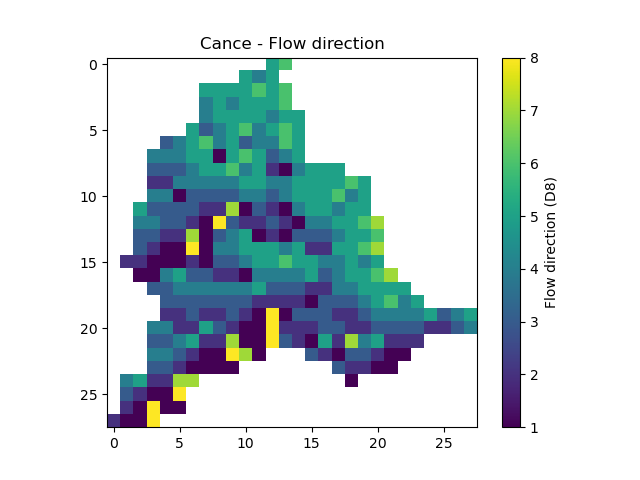
• flwdir

  The flow direction that can be simply visualized that way

  In [13]: plt.imshow(mesh["flwdir"]);
  
  In [14]: plt.colorbar(label="Flow direction (D8)");
  
  In [15]: plt.title("Cance - Flow direction");
  

  

Hint

If the plot is not displayed, try the plt.show() command.

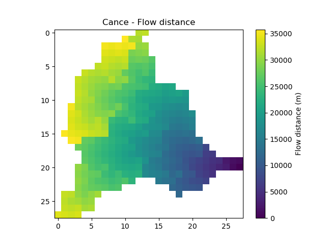
• flwdst

  The flow distance in meter from the most downstream outlet

  In [16]: plt.imshow(mesh["flwdst"]);
  
  In [17]: plt.colorbar(label="Flow distance (m)");
  
  In [18]: plt.title("Cance - Flow distance");
  

  

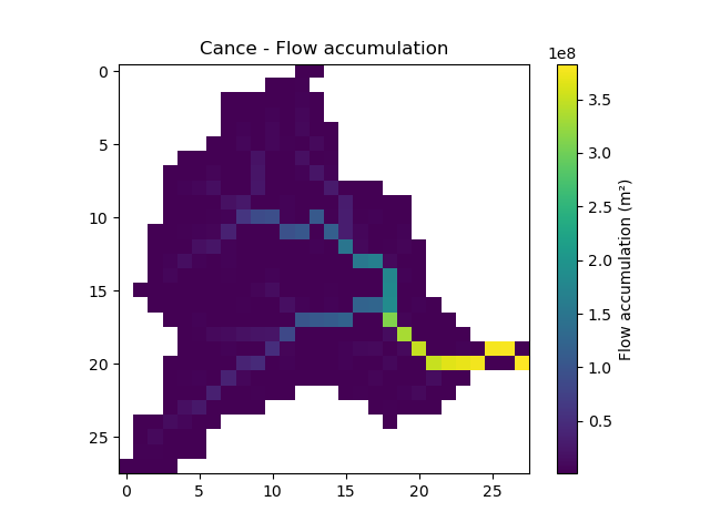
• flwacc

  The flow accumulation in square meter

  In [19]: plt.imshow(mesh["flwacc"]);
  
  In [20]: plt.colorbar(label="Flow accumulation (m²)");
  
  In [21]: plt.title("Cance - Flow accumulation");
  

  

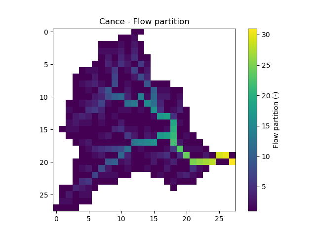
• npar, ncpar, cscpar, cpar_to_rowcol, flwpar

  All the variables related to independent routing partitions. We won’t go into too much detail about these variables, as they simply allow us, in parallel computation, to identify which are the independent cells in the drainage network.

  In [22]: mesh["npar"], mesh["ncpar"], mesh["cscpar"], mesh["cpar_to_rowcol"]
  Out[22]: 
  (np.int32(31),
   array([408, 145,  67,  36,  23,  16,  13,  10,   6,   6,   5,   5,   4,
            4,   4,   4,   4,   4,   3,   3,   3,   2,   1,   1,   1,   1,
            1,   1,   1,   1,   1], dtype=int32),
   array([  0, 408, 553, 620, 656, 679, 695, 708, 718, 724, 730, 735, 740,
          744, 748, 752, 756, 760, 764, 767, 770, 773, 775, 776, 777, 778,
          779, 780, 781, 782, 783], dtype=int32),
   array([[ 3,  0],
          [ 4,  0],
          [ 8,  0],
          ...,
          [19, 25],
          [19, 26],
          [20, 27]], shape=(784, 2), dtype=int32))
  
  In [23]: plt.imshow(mesh["flwpar"]);
  
  In [24]: plt.colorbar(label="Flow partition (-)");
  
  In [25]: plt.title("Cance - Flow partition");
  

  

• nac, active_cell

  The number of active cells, nac and the mask of active cells, active_cell. When meshing, we define a rectangular area of shape (nrow, ncol) in which only a certain number of cells contribute to the discharge at the mesh gauges. This saves us computing time and memory.

  In [26]: mesh["nac"]
  Out[26]: np.int64(383)
  
  In [27]: plt.imshow(mesh["active_cell"]);
  
  In [28]: plt.colorbar(label="Active cell (-)");
  
  In [29]: plt.title("Cance - Active cell");
  

  

• ng, gauge_pos, code, area, area_dln

  All the variables related to the gauges. The number of gauges, ng, the gauges position in terms of rows and columns, gauge_pos, the gauges code, code, the “real” drainage area, area and the delineated drainage area, area_dln.

  In [30]: mesh["ng"], mesh["gauge_pos"], mesh["code"], mesh["area"], mesh["area_dln"]
  Out[30]: 
  (3,
   array([[20, 27],
          [10, 13],
          [ 8, 14]], dtype=int32),
   array(['V3524010', 'V3515010', 'V3517010'], dtype='<U8'),
   array([3.817e+08, 1.070e+08, 2.530e+07], dtype=float32),
   array([3.83e+08, 1.08e+08, 2.80e+07], dtype=float32))
  

Validation of mesh generation

An important step after generating the mesh is to check that the stations have been correctly placed on the flow direction map. To do this, we can try to visualize on which cell each station is located and whether the delineated drainage area is close to the “real” drainage area entered.

In [31]: base = np.zeros(shape=(mesh["nrow"], mesh["ncol"]))

In [32]: base = np.where(mesh["active_cell"] == 0, np.nan, base)

In [33]: for pos in mesh["gauge_pos"]:
   ....:     base[pos[0], pos[1]] = 1
   ....: 

In [34]: plt.imshow(base, cmap="Set1_r");

In [35]: plt.title("Cance - Gauge position");

In [36]: (mesh["area"] - mesh["area_dln"]) / mesh["area"] * 100 # Relative error in %
Out[36]: array([ -0.34058163,  -0.93457943, -10.671937  ], dtype=float32)

For this mesh, we have a negative relative error on the simulated drainage area that varies from -0.3% for the most downstream gauge to -10% for the most upstream one (which can be explained by the fact that small upstream catchments are more sensitive to the relatively coarse mesh resolution).

Saving the mesh

To avoid regenerating the mesh for each simulation with the same case study, we can save it using the smash.io.save_mesh function. This function stores the mesh in an HDF5 file, which can later be read back using the smash.io.read_mesh function.

In [37]: smash.io.save_mesh(mesh, "mesh.hdf5")

In [38]: mesh = smash.io.read_mesh("mesh.hdf5")

In [39]: mesh.keys()
Out[39]: dict_keys(['active_cell', 'area', 'area_dln', 'code', 'cpar_to_rowcol', 'cscpar', 'dx', 'dy', 'flwacc', 'flwdir', 'flwdst', 'flwpar', 'gauge_pos', 'ncpar', 'nac', 'ncol', 'ng', 'npar', 'nrow', 'xmin', 'xres', 'ymax', 'yres'])

Hint

The meshes of demo data in smash can also be loaded using the function smash.factory.load_dataset.