Forward Run and Classical Calibration

This tutorial explains how to perform simple simulations such as a forward run and a simple model optimization. We begin by opening a Python interface:

python3

Imports

We will first import the necessary libraries for this tutorial.

>>> import smash
>>> import matplotlib.pyplot as plt

Hint

The visualization library matplotlib is not installed by default but can be installed with pip as follows:

pip install matplotlib

Model creation

To create a Model object, we need to define both the setup and mesh dictionaries (see the tutorial on Model Object Initialization). For simplificity, starting from this tutorial, we will use the smash.factory.load_dataset function to load the setup and mesh dictionaries.

In this tutorial, we will use the Cance dataset as an example.

>>> setup, mesh = smash.factory.load_dataset("Cance")
>>> model = smash.Model(setup, mesh)

Model simulation

Different methods associated with the Model object are available to perform a simulation such as a forward run or an optimization.

Forward run

The most basic simulation possible is the forward run, which consists of running a forward hydrological model given input data. A forward run can be performed with the Model.forward_run method, which performs an in-place operation on the Model object, or with smash.forward_run, which creates a copy of the Model object.

>>> model.forward_run()  # in-place operation

</> Forward Run

Once the forward run has been completed, we can visualize the simulated discharge, for example, at the most downstream gauge.

>>> code = model.mesh.code[0]
>>> plt.plot(model.response_data.q[0, :], label="Observed discharge")
>>> plt.plot(model.response.q[0, :], label="Simulated discharge")
>>> plt.xlabel("Time step")
>>> plt.ylabel("Discharge ($m^3/s$)")
>>> plt.grid(ls="--", alpha=.7)
>>> plt.legend()
>>> plt.title(f"Observed and simulated discharge at gauge {code}")
>>> plt.show()

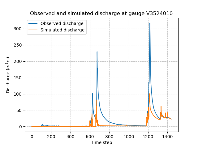
As the hydrograph shows, the simulated discharge is quite different from the observed discharge at this gauge. Obviously, we ran a forward run with the default smash rainfall-runoff parameter set. We can now try to run an optimization to minimize the misfit between the simulated and observed discharge.

Optimization

Similar to the forward run, there are two ways to perform an optimization using either Model.optimize or smash.optimize. The hydrological model optimization problem is complex, and there are many strategies that can be employed depending on the modeling goals and data available. Here, for this first tutorial on model optimization, we consider a simple method with the default optimization parameters. The default cost function J to be minimized here is one minus the Nash-Sutcliffe efficiency (\(1 - \text{NSE}\)), using a global Step-By-Step algorithm (see SBS in Optimization Algorithms). By default, the optimized parameters are supposed to be spatially uniform, which are conceptual rainfall-runoff parameters (here we consider a classical structure with the parameters: cp, ct, kexc, and llr).

>>> model.optimize()
>>> # Equivalent to model.optimize(mapping="uniform", optimizer="sbs")

</> Optimize
    At iterate     0    nfg =     1    J = 6.95010e-01    ddx = 0.64
    At iterate     1    nfg =    30    J = 9.84102e-02    ddx = 0.64
    At iterate     2    nfg =    59    J = 4.54091e-02    ddx = 0.32
    At iterate     3    nfg =    88    J = 3.81819e-02    ddx = 0.16
    At iterate     4    nfg =   117    J = 3.73623e-02    ddx = 0.08
    At iterate     5    nfg =   150    J = 3.70871e-02    ddx = 0.02
    At iterate     6    nfg =   183    J = 3.68001e-02    ddx = 0.02
    At iterate     7    nfg =   216    J = 3.67631e-02    ddx = 0.01
    At iterate     8    nfg =   240    J = 3.67280e-02    ddx = 0.01
    CONVERGENCE: DDX < 0.01

The outputs above show the different iterations of the optimization process, including information on the number of iterations, the cumulative number of evaluations nfg (the number of forward runs performed within each iteration of the optimization algorithm), the value of the cost function J to be minimized, and the value of the adaptive descent step ddx of the heuristic search algorithm. The final message indicates the termination type of the optimization (e.g., converged, stopped by maximum iterations, etc.).

Hint

The default optimization options depend on the chosen mapping and optimizer. To get these default options, use smash.default_optimize_options for smash.optimize, and smash.default_bayesian_optimize_options for smash.bayesian_optimize. For example, the default options for the smash.optimize method using uniform mapping and the SBS optimizer are:

>>> optimize_options = smash.default_optimize_options(model)
>>> # Equivalent to smash.default_optimize_options(model, mapping="uniform", optimizer="sbs")
>>> optimize_options

{'parameters': ['cp', 'ct', 'kexc', 'llr'], 'bounds': {'cp': (1e-06, 1000.0), 'ct': (1e-06, 1000.0), 'kexc': (-50, 50), 'llr': (1e-06, 1000.0)}, 'control_tfm': 'sbs', 'termination_crit': {'maxiter': 50}}

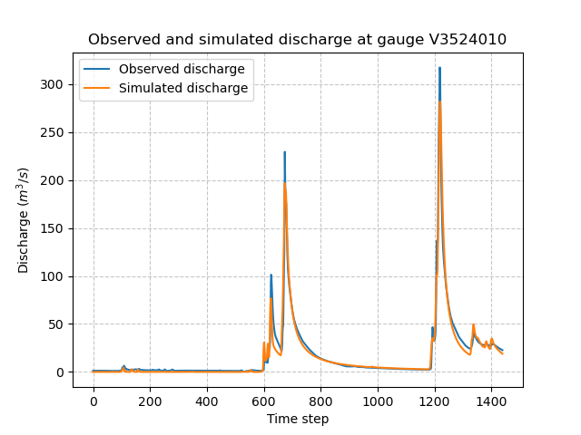
Now, we visualize again the simulated discharge compared to the observed discharge, but this time with optimized model parameters.

>>> code = model.mesh.code[0]
>>> plt.plot(model.response_data.q[0, :], label="Observed discharge")
>>> plt.plot(model.response.q[0, :], label="Simulated discharge")
>>> plt.xlabel("Time step")
>>> plt.ylabel("Discharge ($m^3/s$)")
>>> plt.grid(ls="--", alpha=.7)
>>> plt.legend()
>>> plt.title(f"Observed and simulated discharge at gauge {code}")
>>> plt.show()

We get the optimized values of the rainfall-runoff parameters.

>>> ind = tuple(model.mesh.gauge_pos[0, :])
>>> opt_parameters = {
...     k: model.get_rr_parameters(k)[ind] for k in ["cp", "ct", "kexc", "llr"]
... } # A dictionary comprehension
>>> opt_parameters

{'cp': np.float32(75.816666), 'ct': np.float32(255.8543), 'kexc': np.float32(-1.3692871), 'llr': np.float32(30.552221)}

Note

Hydrological models are often calibrated using a warm-up period to reduce the influence of initial conditions on the optimization process. This period is excluded from the cost function calculation. By default, the start and end times for optimization are set as defined in Model.setup.

>>> model.setup.start_time, model.setup.end_time

('2014-09-15 00:00', '2014-11-14 00:00')

To specify the end of the warm-up period (i.e., the start time for optimization), define the key 'end_warmup' in the cost_options dictionary.

>>> # Optimize Model with a warm-up period
>>> model.optimize(cost_options={"end_warmup": "2014-10-01"})

Save the Model

Finally, the Model object, including all input data and optimized parameters, can be saved to a HDF5 file, and read back using the smash.io.save_model and smash.io.read_model functions.

>>> smash.io.save_model(model, "model.hdf5")
>>> model = smash.io.read_model("model.hdf5")
>>> model

Model
    atmos_data: ['mean_pet', 'mean_prcp', '...', 'sparse_prcp', 'sparse_snow']
    mesh: ['active_cell', 'area', '...', 'xres', 'ymax']
    nn_parameters: ['bias_1', 'bias_2', '...', 'weight_1', 'weight_2']
    physio_data: ['descriptor', 'imperviousness', 'l_descriptor', 'u_descriptor']
    response: ['q']
    response_data: ['q']
    rr_final_states: ['keys', 'values']
    rr_initial_states: ['keys', 'values']
    rr_parameters: ['keys', 'values']
    serr_mu_parameters: ['keys', 'values']
    serr_sigma_parameters: ['keys', 'values']
    setup: ['adjust_interception', 'compute_mean_atmos', '...', 'temp_access', 'temp_directory']
    u_response_data: ['q_stdev']

Hint

For large domain simulations, the model object can be quite large. An alternative, lighter solution is to use the smash.io.save_model_ddt and smash.io.read_model_ddt functions. This method saves important derived data types of the Model object to the HDF5 file instead of the entire Model object. However, there is no smash method to reconstruct the Model object from this saved data file.

>>> smash.io.save_model_ddt(model, "model_ddt.hdf5")
>>> model_ddt = smash.io.read_model_ddt("model_ddt.hdf5")
>>> model_ddt.keys()  # a dictionary containing several derived data types of the Model object

dict_keys(['mesh', 'nn_parameters', 'physio_data', 'response', 'response_data', 'rr_final_states', 'rr_initial_states', 'rr_parameters', 'serr_mu_parameters', 'serr_sigma_parameters', 'setup'])