Split Sample and Temporal Validation#

The objective of this tutorial is to learn how to set up an optimization with a split sample test [Klemeš, 1986] in smash, i.e., cross-calibration and temporal validation over two distinct periods p1 and p2.

Open a Python interface:

python3

Imports#

We will first import the necessary libraries for this tutorial.

>>> import smash
>>> import numpy as np
>>> import pandas as pd
>>> import matplotlib.pyplot as plt

Model creation#

In this tutorial, we will use the Lez dataset as an example.

>>> setup, mesh = smash.factory.load_dataset("lez")

Check the start and end time defined in the setup:

>>> setup["start_time"], setup["end_time"]

(datetime.date(2012, 8, 1), datetime.date(2013, 7, 31))

Since we are going to work on two different periods, each of 6 months, we need to create two setup dictionaries where the only difference will be in the simulation period arguments start_time and end_time. The first period p1 will run from 2012-08-01 to 2013-01-31 and the second, from 2013-02-01 to 2013-07-31.

>>> setup_p1 = setup.copy()
>>> setup_p1.update(
...     {
...         "start_time": "2012-08-01",
...         "end_time": "2013-01-31",
...     }
... )
>>>
>>> setup_p2 = setup.copy()
>>> setup_p2.update(
...     {
...         "start_time": "2013-02-01",
...         "end_time": "2013-07-31",
...     }
... )

For the mesh, there is no need to generate two different mesh dictionaries, the same one can be used for both time periods. Now we can initialize the two smash.Model objects:

>>> model_p1 = smash.Model(setup_p1, mesh)
>>> model_p2 = smash.Model(setup_p2, mesh)

Model calibration and validation#

Optimization#

First, we will optimize both models for each period to generate two sets of optimized rainfall-runoff parameters. So far, to optimize, we have called the method associated with the smash.Model object Model.optimize. This method will modify the associated object in place (i.e., the values of the rainfall-runoff parameters after calling this function are modified). Here, we want to optimize the model but still keep this model object to run the validation afterwards. To do this, instead of calling the Model.optimize method, we can call the smash.optimize function, which is identical but takes a smash.Model object as input and returns a copy of it. This method allows you to optimize a smash.Model object and store the results in another object without modifying the initial one.

Here, we perform a simple derivative-free optimization algorithm, for instance SBS (see Optimization Algorithms), to optimize the spatially uniform hydrological parameters. We use a default cost function equal to one minus the Nash-Sutcliffe efficiency at the most downstream gauge.

>>> model_p1_opt = smash.optimize(model_p1)

</> Optimize
    At iterate     0    nfg =     1    J = 1.35661e+00    ddx = 0.64
    At iterate     1    nfg =    30    J = 8.30659e-01    ddx = 0.64
    At iterate     2    nfg =    58    J = 4.63114e-01    ddx = 0.32
    At iterate     3    nfg =    88    J = 4.00084e-01    ddx = 0.16
    At iterate     4    nfg =   117    J = 3.93997e-01    ddx = 0.08
    At iterate     5    nfg =   151    J = 3.87771e-01    ddx = 0.04
    At iterate     6    nfg =   183    J = 3.82824e-01    ddx = 0.04
    At iterate     7    nfg =   215    J = 3.78023e-01    ddx = 0.08
    At iterate     8    nfg =   248    J = 3.68680e-01    ddx = 0.08
    At iterate     9    nfg =   281    J = 3.63157e-01    ddx = 0.16
    At iterate    10    nfg =   316    J = 3.58884e-01    ddx = 0.08
    At iterate    11    nfg =   349    J = 3.58221e-01    ddx = 0.04
    At iterate    12    nfg =   383    J = 3.56019e-01    ddx = 0.04
    At iterate    13    nfg =   416    J = 3.55442e-01    ddx = 0.02
    At iterate    14    nfg =   451    J = 3.54573e-01    ddx = 0.02
    At iterate    15    nfg =   477    J = 3.54552e-01    ddx = 0.01
    CONVERGENCE: DDX < 0.01

>>> model_p2_opt = smash.optimize(model_p2)

</> Optimize
    At iterate     0    nfg =     1    J = 1.27190e+00    ddx = 0.64
    At iterate     1    nfg =    30    J = 4.14639e-01    ddx = 0.64
    At iterate     2    nfg =    58    J = 3.22555e-01    ddx = 0.64
    At iterate     3    nfg =    87    J = 1.80229e-01    ddx = 0.64
    At iterate     4    nfg =   115    J = 1.71559e-01    ddx = 0.64
    At iterate     5    nfg =   149    J = 1.53549e-01    ddx = 1.28
    At iterate     6    nfg =   181    J = 1.52750e-01    ddx = 1.28
    At iterate     7    nfg =   214    J = 1.52746e-01    ddx = 0.32
    At iterate     8    nfg =   250    J = 1.44511e-01    ddx = 0.08
    At iterate     9    nfg =   285    J = 1.44496e-01    ddx = 0.02
    At iterate    10    nfg =   318    J = 1.44471e-01    ddx = 0.01
    CONVERGENCE: DDX < 0.01

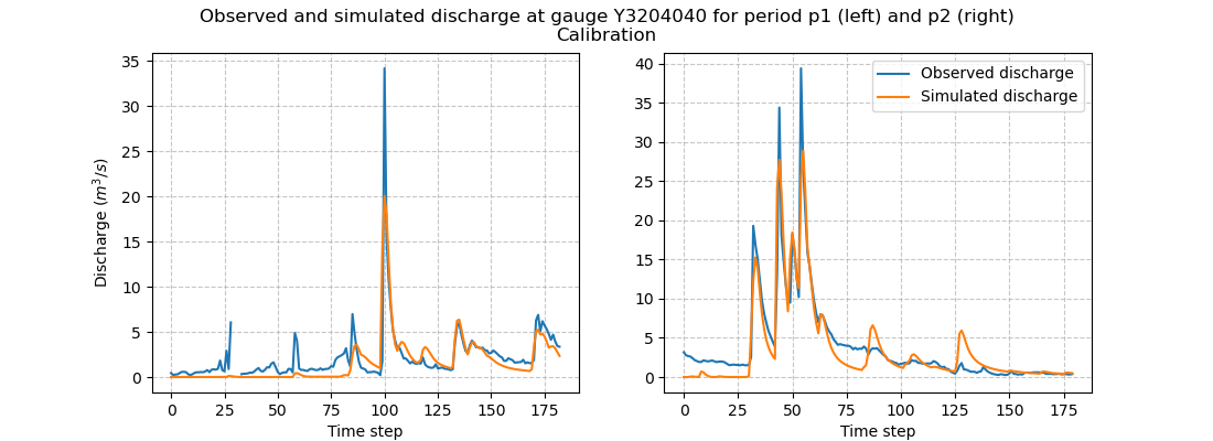
We can take a look at the hydrographs and the optimized rainfall-runoff parameters.

>>> code = model_p1.mesh.code[0]
>>>
>>> f, (ax1, ax2) = plt.subplots(1, 2, figsize=(11, 4))
>>>
>>> qobs = model_p1_opt.response_data.q[0,:].copy()
>>> qobs = np.where(qobs < 0, np.nan, qobs) # To deal with missing values
>>> qsim = model_p1_opt.response.q[0,:]
>>> ax1.plot(qobs)
>>> ax1.plot(qsim)
>>> ax1.grid(ls="--", alpha=.7)
>>> ax1.set_xlabel("Time step")
>>> ax1.set_ylabel("Discharge ($m^3/s$)")
>>>
>>> qobs = model_p2_opt.response_data.q[0,:].copy()
>>> qobs = np.where(qobs < 0, np.nan, qobs) # To deal with missing values
>>> qsim = model_p2_opt.response.q[0,:]
>>> ax2.plot(qobs, label="Observed discharge")
>>> ax2.plot(qsim, label="Simulated discharge")
>>> ax2.grid(ls="--", alpha=.7)
>>> ax2.set_xlabel("Time step")
>>> ax2.legend()
>>>
>>> f.suptitle(
...     f"Observed and simulated discharge at gauge {code}"
...     " for period p1 (left) and p2 (right)\nCalibration"
... )
>>> plt.show()

../../_images/user_guide.classical_uses.split_sample_temporal_validation.optimize_q.png

>>> ind = tuple(model_p1.mesh.gauge_pos[0, :])
>>>
>>> opt_parameters_p1 = {
...     k: model_p1_opt.get_rr_parameters(k)[ind] for k in ["cp", "ct", "kexc", "llr"]
... }
>>> opt_parameters_p1

{'cp': np.float32(160.68974), 'ct': np.float32(35.321835), 'kexc': np.float32(0.017074872), 'llr': np.float32(557.58215)}

>>> opt_parameters_p2 = {
...     k: model_p2_opt.get_rr_parameters(k)[ind] for k in ["cp", "ct", "kexc", "llr"]
... }
>>> opt_parameters_p2

{'cp': np.float32(9.942335e-05), 'ct': np.float32(107.30205), 'kexc': np.float32(-2.3589046), 'llr': np.float32(498.9533)}

Temporal validation#

Rainfall-runoff parameters transfer#

We can now transfer the optimized rainfall-runoff parameters for each calibration period to the respective validation period. We will transfer the rainfall-runoff parameters from model_p1_opt to model_p2 and from model_p2_opt to model_p1. There are several ways to do this:

Transfer all rainfall-runoff parameters at once
All rainfall-runoff parameters are stored in the variable values of the object Model.rr_parameters. We can therefore pass the whole array of rainfall-runoff parameters from one object to the other.
>>> model_p1.rr_parameters.values = model_p2_opt.rr_parameters.values.copy() >>> model_p2.rr_parameters.values = model_p1_opt.rr_parameters.values.copy()
Note

A deep copy is recommended to avoid that the rainfall-runoff parameters between each object become shallow copies and so that the modification of one of the arrays leads to the modification of another.
Transfer each rainfall-runoff parameter one by one
It is also possible to loop on each rainfall-runoff parameter and assign new rainfall-runoff parameter by passing by getters and setters
>>> for key in model_p1.rr_parameters.keys: ... model_p1.set_rr_parameters(key, model_p2_opt.get_rr_parameters(key)) ... model_p2.set_rr_parameters(key, model_p1_opt.get_rr_parameters(key))
Note

This method allows, instead of looping on all rainfall-runoff parameters, to loop only on some. We can replace model_p1.rr_parameters.keys by ["cp", "ct"] for example

Forward run#

Once the rainfall-runoff parameters have been transferred, we can proceed with the validation forward runs by calling the Model.forward_run method.

>>> model_p1.forward_run()
>>> model_p2.forward_run()

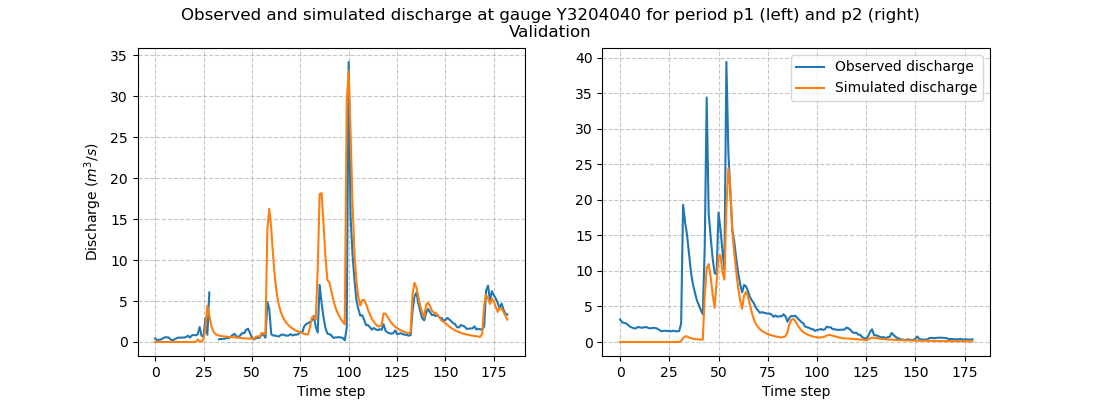
and visualize the hydrographs:

>>> code = model_p1.mesh.code[0]
>>>
>>> f, (ax1, ax2) = plt.subplots(1, 2, figsize=(11, 4));
>>>
>>> qobs = model_p1.response_data.q[0,:].copy()
>>> qobs = np.where(qobs < 0, np.nan, qobs) # To deal with missing values
>>> qsim = model_p1.response.q[0,:]
>>> ax1.plot(qobs)
>>> ax1.plot(qsim)
>>> ax1.grid(ls="--", alpha=.7)
>>> ax1.set_xlabel("Time step")
>>> ax1.set_ylabel("Discharge ($m^3/s$)")
>>>
>>> qobs = model_p2.response_data.q[0,:].copy()
>>> qobs = np.where(qobs < 0, np.nan, qobs) # To deal with missing values
>>> qsim = model_p2.response.q[0,:]
>>> ax2.plot(qobs, label="Observed discharge")
>>> ax2.plot(qsim, label="Simulated discharge")
>>> ax2.grid(ls="--", alpha=.7)
>>> ax2.set_xlabel("Time step")
>>> ax2.legend()
>>>
>>> f.suptitle(
...     f"Observed and simulated discharge at gauge {code}"
...     " for period p1 (left) and p2 (right)\nValidation"
... )
>>> plt.show()

../../_images/user_guide.classical_uses.split_sample_temporal_validation.forward_run_q.png

Scoring metrics#

We evaluate calibration and validation performances using certain metrics. Using the function smash.evaluation, you can compute one metric of your choice (among those available) for all the gauges that make up the mesh. Here, we are interested in the nse (the calibration metric) and the kge for the downstream gauge only. We will create two pandas.DataFrame, one for the calibration performances and the other for the validation performances.

>>> metrics = ["NSE", "KGE"]
>>> perf_cal = pd.DataFrame(index=["p1", "p2"], columns=metrics)
>>> perf_val = perf_cal.copy()
>>>
>>> perf_cal.loc["p1"] = np.round(smash.evaluation(model_p1_opt, metrics)[0, :], 2)
>>> perf_cal.loc["p2"] = np.round(smash.evaluation(model_p2_opt, metrics)[0, :], 2)
>>>
>>> perf_val.loc["p1"] = np.round(smash.evaluation(model_p1, metrics)[0, :], 2)
>>> perf_val.loc["p2"] = np.round(smash.evaluation(model_p2, metrics)[0, :], 2)

Calibration performances:

>>> perf_cal

     NSE   KGE
p1  0.65   0.7
p2  0.86  0.88

Validation performances:

>>> perf_val

     NSE   KGE
p1 -0.38  0.17
p2  0.53  0.35