Improving the first guess using Bayesian estimation

Here, we aim to improve the spatially uniform first guess using the Bayesian estimation approach.

To get started, open a Python interface:

python3

Imports

In [1]: import smash

In [2]: import matplotlib.pyplot as plt

In [3]: import numpy as np

Model object creation

First, you need to create a smash.Model object. For this case, we will use the Lez dataset.

Load the setup and mesh dictionaries using the smash.load_dataset() method and create the smash.Model object.

In [4]: setup, mesh = smash.load_dataset("Lez")

In [5]: model = smash.Model(setup, mesh)

LDBE (Low Dimensional Bayesian Estimation)

Next, we find a uniform first guess using Bayesian estimation on a random set of the Model parameters using the smash.Model.bayes_estimate() method. By default, the sample argument is not required to be set, and it is automatically set based on the Model structure. This example shows how to define a custom sample using the smash.generate_samples() method.

You may refer to the smash.Model.get_bound_constraints() method to obtain some information about the Model parameters/states:

In [6]: model.get_bound_constraints()
Out[6]: 
{'num_vars': 4,
 'names': ['cp', 'cft', 'exc', 'lr'],
 'bounds': [[9.999999974752427e-07, 1000.0],
  [9.999999974752427e-07, 1000.0],
  [-50.0, 50.0],
  [9.999999974752427e-07, 1000.0]]}

Here we define a problem that only contains three Model parameters, which means the fourth one will be fixed:

In [7]: problem = {
   ...:         "num_vars": 3,
   ...:         "names": ["cp", "lr", "cft"],
   ...:         "bounds": [[1, 1000], [1, 1000], [1, 1000]]
   ...:     }
   ...: 

We then generate a set of 400 random Model parameters:

In [8]: sr = smash.generate_samples(problem, n=400, random_state=1)

and perform Bayesian estimation:

In [9]: model_be, br = model.bayes_estimate(sr, alpha=np.linspace(-1, 4, 50), return_br=True);

In [10]: model_be.output.cost  # cost value with LDBE
Out[10]: 0.19659416377544403

In the code above, we used the L-curve approach to find an optimal regularization parameter within a short search range of \([-1, 4]\).

Visualization of estimation results

Now, we can use the br instance of smash.BayesResult to visualize information about the estimation process. For example, we can plot the distribution of cost values obtained from running the forward hydrological model with the random set of parameters using the following code:

In [11]: plt.hist(br.data["cost"], bins=30, zorder=2);

In [12]: plt.grid(alpha=.7, ls="--", zorder=1);

In [13]: plt.xlabel("Cost");

In [14]: plt.ylabel("Frequency");

In [15]: plt.title("Cost value histogram for parameter set");

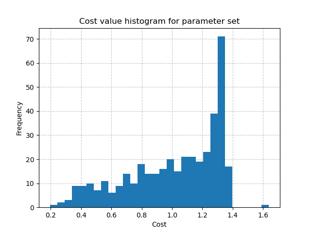
The minimal cost value through the forward runs:

In [16]: np.min(br.data["cost"])
Out[16]: 0.19453579187393188

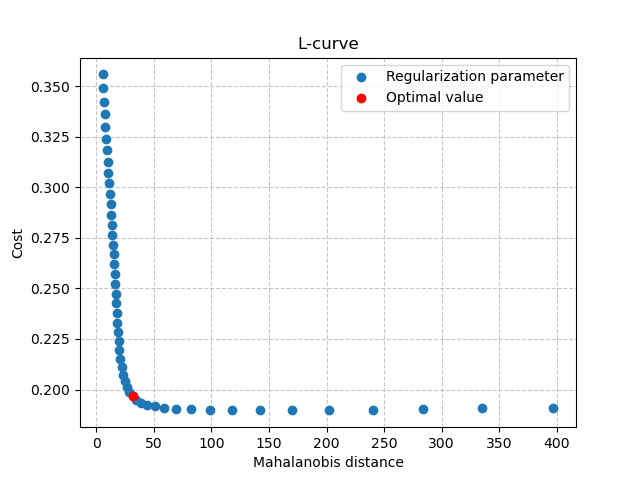
We can also visualize the L-curve that was used to find the optimal regularization parameter:

In [17]: opt_ind = np.where(br.lcurve["alpha"]==br.lcurve["alpha_opt"])[0][0]

In [18]: plt.scatter(
   ....:         br.lcurve["mahal_dist"],
   ....:         br.lcurve["cost"],
   ....:         label="Regularization parameter",
   ....:         zorder=2
   ....:     );
   ....: 

In [19]: plt.scatter(
   ....:         br.lcurve["mahal_dist"][opt_ind],
   ....:         br.lcurve["cost"][opt_ind],
   ....:         color="red",
   ....:         label="Optimal value",
   ....:         zorder=3
   ....:     );
   ....: 

In [20]: plt.grid(alpha=.7, ls="--", zorder=1);

In [21]: plt.xlabel("Mahalanobis distance");

In [22]: plt.ylabel("Cost");

In [23]: plt.title("L-curve");

In [24]: plt.legend();

The spatially uniform first guess:

In [25]: ind = tuple(model_be.mesh.gauge_pos[0,:])

In [26]: ind
Out[26]: (26, 12)

In [27]: (
   ....:  model_be.parameters.cp[ind],
   ....:  model_be.parameters.cft[ind],
   ....:  model_be.parameters.exc[ind],
   ....:  model_be.parameters.lr[ind],
   ....: )
   ....: 
Out[27]: (112.33628, 99.58623, 0.0, 518.99603)

Comparing to the initial values of the parameters:

In [28]: (
   ....:  model.parameters.cp[ind],
   ....:  model.parameters.cft[ind],
   ....:  model.parameters.exc[ind],
   ....:  model.parameters.lr[ind],
   ....: )
   ....: 
Out[28]: (200.0, 500.0, 0.0, 120.0)

We can see that the value of exc did not change since it is not set to be estimated.

Variational calibration using Bayesian estimation first guess

Finally, we perform a variational calibration on the Model parameters using the \(\mathrm{L}\text{-}\mathrm{BFGS}\text{-}\mathrm{B}\) algorithm and the Bayesian first guess:

In [29]: model_sd = model_be.optimize(
   ....:     mapping="distributed",
   ....:     algorithm="l-bfgs-b",
   ....:     options={"maxiter": 30}
   ....: )
   ....: 

In [30]: model_sd.output.cost  # the cost value
Out[30]: 0.12787534296512604

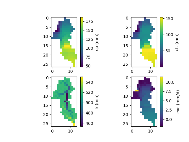
The spatially distributed model parameters:

In [31]: ma = (model_sd.mesh.active_cell == 0)

In [32]: ma_cp = np.where(ma, np.nan, model_sd.parameters.cp)

In [33]: ma_cft = np.where(ma, np.nan, model_sd.parameters.cft)

In [34]: ma_lr = np.where(ma, np.nan, model_sd.parameters.lr)

In [35]: ma_exc = np.where(ma, np.nan, model_sd.parameters.exc)

In [36]: f, ax = plt.subplots(2, 2)

In [37]: map_cp = ax[0,0].imshow(ma_cp);

In [38]: f.colorbar(map_cp, ax=ax[0,0], label="cp (mm)");

In [39]: map_cft = ax[0,1].imshow(ma_cft);

In [40]: f.colorbar(map_cft, ax=ax[0,1], label="cft (mm)");

In [41]: map_lr = ax[1,0].imshow(ma_lr);

In [42]: f.colorbar(map_lr, ax=ax[1,0], label="lr (min)");

In [43]: map_exc = ax[1,1].imshow(ma_exc);

In [44]: f.colorbar(map_exc, ax=ax[1,1], label="exc (mm/d)");