Multi-criteria optimization

Here, we aim to optimize the Model parameters/states using multiple calibration metrics based on certain hydrological signatures.

To get started, open a Python interface:

python3

Imports

In [1]: import smash

In [2]: import matplotlib.pyplot as plt

Model object creation

First, you need to create a smash.Model object. For this case, we will use the Lez dataset.

Load the setup and mesh dictionaries using the smash.load_dataset() method and create the smash.Model object.

In [3]: setup, mesh = smash.load_dataset("Lez")

In [4]: model = smash.Model(setup, mesh)

Multiple metrics calibration using signatures

This method enables the incorporation of multiple calibration metrics into the observation term of the cost function (for mathematical details, see the Math / Num Documentation section). Hydrological signatures are thus introduced to tackle such an approach. Note that this multi-criteria approach is possible for all optimization methods, including smash.Model.optimize(), smash.Model.bayes_estimate(), smash.Model.bayes_optimize() and smash.Model.ann_optimize(). For simplicity, in this example, we use smash.Model.optimize() with a uniform mapping.

Let us consider a classical calibration with a single metric:

In [5]: model_sm = model.optimize(jobs_fun="nse");

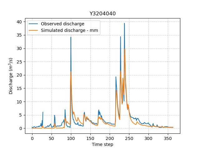
Now we employ, for instance, continuous and flood-event runoff coefficients (Crc and Erc) for multi-criteria calibration:

In [6]: model_mm = model.optimize(jobs_fun=["nse", "Crc", "Erc"], wjobs_fun=[0.6, 0.1, 0.3]);

where the weights of the objective functions based on nse, Crc, Erc are set to 0.6, 0.1 and 0.3 respectively. If these weights are not given by user, the cost value is computed as the mean of the objective functions.

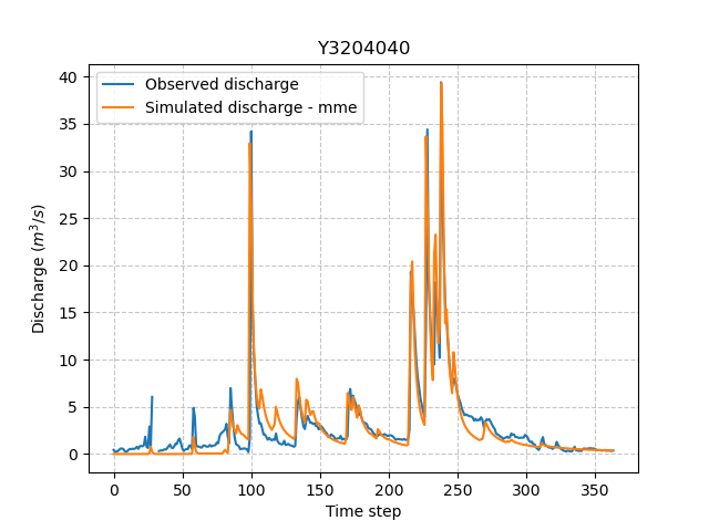
For multiple metrics calibration based on flood-event signatures, we can further adjust some parameters in the segmentation algorithm to compute flood-event signatures. For example, we use a multi-criteria cost function based on the peak flow Epf to calibrate the Model parameters:

In [7]: model_mme = model.optimize(
   ...:         jobs_fun=["nse", "Epf"],
   ...:         event_seg={"peak_quant": 0.99},
   ...:         wjobs_fun=[0.6, 0.4]
   ...:     )
   ...: 

Finally, the simulated discharges of the three models can be visualized as follows:

In [8]: qo = model.input_data.qobs[0,:].copy()

In [9]: qo = np.where(qo<0, np.nan, qo)  # to deal with missing data

In [10]: plt.plot(qo, label="Observed discharge");

In [11]: plt.plot(model_sm.output.qsim[0,:], label="Simulated discharge - sm");

In [12]: plt.grid(alpha=.7, ls="--");

In [13]: plt.xlabel("Time step");

In [14]: plt.ylabel("Discharge $(m^3/s)$");

In [15]: plt.title(model_mm.mesh.code[0]);

In [16]: plt.legend();

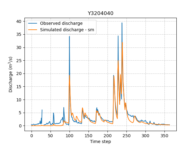
In [17]: plt.plot(qo, label="Observed discharge");

In [18]: plt.plot(model_mm.output.qsim[0,:], label="Simulated discharge - mm");

In [19]: plt.grid(alpha=.7, ls="--");

In [20]: plt.xlabel("Time step");

In [21]: plt.ylabel("Discharge $(m^3/s)$");

In [22]: plt.title(model_mm.mesh.code[0]);

In [23]: plt.legend();

In [24]: plt.plot(qo, label="Observed discharge");

In [25]: plt.plot(model_mme.output.qsim[0,:], label="Simulated discharge - mme");

In [26]: plt.grid(alpha=.7, ls="--");

In [27]: plt.xlabel("Time step");

In [28]: plt.ylabel("Discharge $(m^3/s)$");

In [29]: plt.title(model_mm.mesh.code[0]);

In [30]: plt.legend();