Pre-regionalization using polynomial mapping

Here, we aim to employ some physiographic descriptors to find the pre-regionalization mapping using polynomial functions. Six descriptors are considered in this example, which are:

• Slope

• Drainage density

• Karst

• Woodland

• Urban

• Soil water storage

First, open a Python interface:

python3

Imports

In [1]: import smash

In [2]: import matplotlib.pyplot as plt

Model object creation

To perform the calibrations, you need to create a smash.Model object. For this case, we will use the Lez dataset.

Load the setup and mesh dictionaries using the smash.load_dataset() method and create the smash.Model object.

In [3]: setup, mesh = smash.load_dataset("Lez")

In [4]: model = smash.Model(setup, mesh)

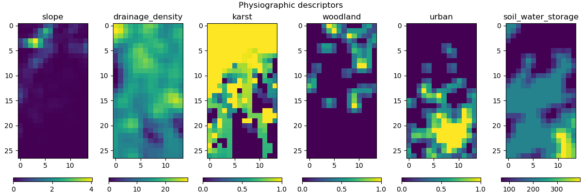
Visualization of descriptors

This method requires input descriptors, which were provided during the creation of the Model object. We can visualize these descriptors and verify if they were successfully loaded:

In [5]: model.input_data.descriptor.shape
Out[5]: (27, 14, 6)

In [6]: desc_name = model.setup.descriptor_name

In [7]: fig, axes = plt.subplots(1, len(desc_name), figsize=(12,4), constrained_layout=True)

In [8]: for i, ax in enumerate(axes):
   ...:     ax.set_title(desc_name[i]);
   ...:     im = ax.imshow(model.input_data.descriptor[..., i]);
   ...:     cbar = fig.colorbar(im, ax=ax, orientation="horizontal");
   ...:     cbar.ax.tick_params();
   ...: 

In [9]: fig.suptitle("Physiographic descriptors");

# Reset figsize to the Matplotlib default
In [10]: plt.figure(figsize=plt.rcParamsDefault['figure.figsize']);

Finding a uniform first guess

Similar to the fully-distributed optimization method, providing a uniform first guess is recommended for this method. In this case, we use the \(\mathrm{SBS}\) algorithm to find such a first guess:

In [11]: model_su = model.optimize(mapping="uniform", algorithm="sbs", options={"maxiter": 2});

Hint

You may want to refer to the Bayesian estimation section for information on how to improve the first guess using a Bayesian estimation approach.

Optimizing hyperparameters for pre-regionalization mapping

There are two types of polynomial mapping that can be employed for pre-regionalization:

• hyper-linear: a linear mapping where the hyperparameters to be estimated are the coefficients.

• hyper-polynomial: a polynomial mapping where the hyperparameters to be estimated are the coefficients and the degree.

As an example, the hyper-polynomial mapping can be combined with the variational calibration algorithm \(\mathrm{L}\text{-}\mathrm{BFGS}\text{-}\mathrm{B}\) as shown below:

In [12]: model_hp = model_su.optimize(
   ....:         mapping="hyper-polynomial",
   ....:         algorithm="l-bfgs-b",
   ....:         options={"maxiter": 30}
   ....:     )
   ....: 

Some information are also provided during the optimization:

</> Optimize Model
    Mapping: 'hyper-polynomial' k(x) = a0 + a1 * D1 ** b1 + ... + an * Dn ** bn
    Algorithm: 'l-bfgs-b'
    Jobs function: [ nse ]
    wJobs: [ 1.0 ]
    Jreg function: 'prior'
    wJreg: 0.000000
    Nx: 1
    Np: 52 [ cp cft exc lr ]
    Ns: 0 [  ]
    Ng: 1 [ Y3204040 ]
    wg: 1 [ 1.0 ]

    At iterate      0    nfg =     1    J =  0.176090    |proj g| =  0.000000
    At iterate      1    nfg =     3    J =  0.174870    |proj g| =  0.160574
    At iterate      2    nfg =     4    J =  0.173283    |proj g| =  0.059085
    At iterate      3    nfg =     5    J =  0.172243    |proj g| =  0.043317
    At iterate      4    nfg =     6    J =  0.171181    |proj g| =  0.045926
    At iterate      5    nfg =     7    J =  0.170460    |proj g| =  0.023084
    At iterate      6    nfg =     8    J =  0.169568    |proj g| =  0.025826
    At iterate      7    nfg =     9    J =  0.168186    |proj g| =  0.046616
    At iterate      8    nfg =    10    J =  0.165931    |proj g| =  0.069842
    At iterate      9    nfg =    11    J =  0.160961    |proj g| =  0.077036
    At iterate     10    nfg =    13    J =  0.152905    |proj g| =  0.209049
    At iterate     11    nfg =    14    J =  0.148905    |proj g| =  0.056703
...
    At iterate     28    nfg =    34    J =  0.133811    |proj g| =  0.008069
    At iterate     29    nfg =    35    J =  0.133753    |proj g| =  0.003290
    At iterate     30    nfg =    36    J =  0.133749    |proj g| =  0.001082
    STOP: TOTAL NO. OF ITERATION EXCEEDS LIMIT

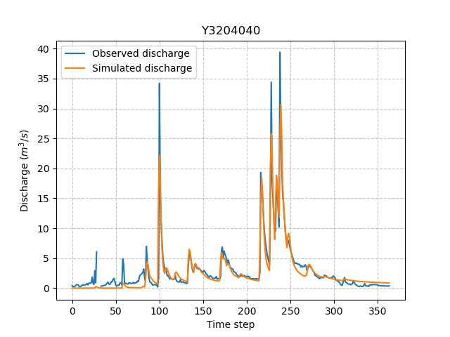
Visualization of results

Now we can visualize the simulated discharge:

In [13]: qo = model_hp.input_data.qobs[0,:].copy()

In [14]: qo = np.where(qo<0, np.nan, qo)  # to deal with missing data

In [15]: plt.plot(qo, label="Observed discharge");

In [16]: plt.plot(model_hp.output.qsim[0,:], label="Simulated discharge");

In [17]: plt.grid(alpha=.7, ls="--");

In [18]: plt.xlabel("Time step");

In [19]: plt.ylabel("Discharge $(m^3/s)$");

In [20]: plt.title(model_hp.mesh.code[0]);

In [21]: plt.legend();

The cost value:

In [22]: model_hp.output.cost
Out[22]: 0.13374879956245422

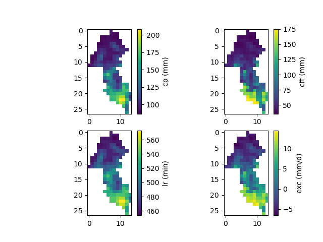
And finally, the spatially distributed model parameters constrained by physiographic descriptors:

In [23]: ma = (model_hp.mesh.active_cell == 0)

In [24]: ma_cp = np.where(ma, np.nan, model_hp.parameters.cp)

In [25]: ma_cft = np.where(ma, np.nan, model_hp.parameters.cft)

In [26]: ma_lr = np.where(ma, np.nan, model_hp.parameters.lr)

In [27]: ma_exc = np.where(ma, np.nan, model_hp.parameters.exc)

In [28]: f, ax = plt.subplots(2, 2)

In [29]: map_cp = ax[0,0].imshow(ma_cp);

In [30]: f.colorbar(map_cp, ax=ax[0,0], label="cp (mm)");

In [31]: map_cft = ax[0,1].imshow(ma_cft);

In [32]: f.colorbar(map_cft, ax=ax[0,1], label="cft (mm)");

In [33]: map_lr = ax[1,0].imshow(ma_lr);

In [34]: f.colorbar(map_lr, ax=ax[1,0], label="lr (min)");

In [35]: map_exc = ax[1,1].imshow(ma_exc);

In [36]: f.colorbar(map_exc, ax=ax[1,1], label="exc (mm/d)");