Fully-distributed optimization using a uniform first guess

To get started, open a Python interface:

python3

Imports

In [1]: import smash

In [2]: import matplotlib.pyplot as plt

In [3]: import numpy as np

Model object creation

To perform the calibrations, you need to create a smash.Model object. For this case, we will use the Lez dataset.

Load the setup and mesh dictionaries using the smash.load_dataset() method and create the smash.Model object.

In [4]: setup, mesh = smash.load_dataset("Lez")

In [5]: model = smash.Model(setup, mesh)

Spatially uniform optimization

To find the uniform first guess, we can perform a spatially-uniform calibration using global optimization algorithms. Here’s an example how we can do it with the \(\mathrm{SBS}\) algorithm:

In [6]: model_su = model.optimize(mapping="uniform", algorithm="sbs", options={"maxiter": 2});

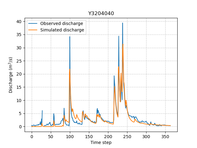
Once the optimization is complete. We can visualize the simulated discharge:

In [7]: qo = model_su.input_data.qobs[0,:].copy()

In [8]: qo = np.where(qo<0, np.nan, qo)  # to deal with missing data

In [9]: plt.plot(qo, label="Observed discharge");

In [10]: plt.plot(model_su.output.qsim[0,:], label="Simulated discharge");

In [11]: plt.grid(alpha=.7, ls="--");

In [12]: plt.xlabel("Time step");

In [13]: plt.ylabel("Discharge $(m^3/s)$");

In [14]: plt.title(model_su.mesh.code[0]);

In [15]: plt.legend();

The cost function value \(J\):

In [16]: model_su.output.cost
Out[16]: 0.17609025537967682

And the spatially uniform first guess:

In [17]: ind = tuple(model_su.mesh.gauge_pos[0,:])

In [18]: ind
Out[18]: (26, 12)

In [19]: (
   ....:  model_su.parameters.cp[ind],
   ....:  model_su.parameters.cft[ind],
   ....:  model_su.parameters.exc[ind],
   ....:  model_su.parameters.lr[ind],
   ....: )
   ....: 
Out[19]: (55.60748, 139.0187, 1.6593012, 431.59668)

Hint

You may want to refer to the Bayesian estimation section for information on how to improve the first guess using a Bayesian estimation approach.

Spatially distributed optimization

Next, using the first guess provided by a global calibration, which had stored the optimized parameters in the previous step, we perform a spatially distributed calibration using the \(\mathrm{L}\text{-}\mathrm{BFGS}\text{-}\mathrm{B}\) algorithm:

In [20]: model_sd = model_su.optimize(
   ....:         mapping="distributed",
   ....:         algorithm="l-bfgs-b",
   ....:         options={"maxiter": 30}
   ....:     )
   ....: 

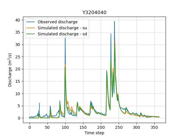
We can once again visualize, the simulated discharges (su: spatially uniform, sd: spatially distributed):

In [21]: qo = model_sd.input_data.qobs[0,:].copy()

In [22]: qo = np.where(qo<0, np.nan, qo)  # to deal with missing data

In [23]: plt.plot(qo, label="Observed discharge");

In [24]: plt.plot(model_su.output.qsim[0,:], label="Simulated discharge - su");

In [25]: plt.plot(model_sd.output.qsim[0,:], label="Simulated discharge - sd");

In [26]: plt.grid(alpha=.7, ls="--");

In [27]: plt.xlabel("Time step");

In [28]: plt.ylabel("Discharge $(m^3/s)$");

In [29]: plt.title(model_sd.mesh.code[0]);

In [30]: plt.legend();

The cost value:

In [31]: model_sd.output.cost
Out[31]: 0.13125108182430267

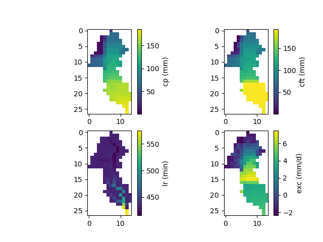
And finally, the distributed model parameters in this case:

In [32]: ma = (model_sd.mesh.active_cell == 0)

In [33]: ma_cp = np.where(ma, np.nan, model_sd.parameters.cp)

In [34]: ma_cft = np.where(ma, np.nan, model_sd.parameters.cft)

In [35]: ma_lr = np.where(ma, np.nan, model_sd.parameters.lr)

In [36]: ma_exc = np.where(ma, np.nan, model_sd.parameters.exc)

In [37]: f, ax = plt.subplots(2, 2)

In [38]: map_cp = ax[0,0].imshow(ma_cp);

In [39]: f.colorbar(map_cp, ax=ax[0,0], label="cp (mm)");

In [40]: map_cft = ax[0,1].imshow(ma_cft);

In [41]: f.colorbar(map_cft, ax=ax[0,1], label="cft (mm)");

In [42]: map_lr = ax[1,0].imshow(ma_lr);

In [43]: f.colorbar(map_lr, ax=ax[1,0], label="lr (min)");

In [44]: map_exc = ax[1,1].imshow(ma_exc);

In [45]: f.colorbar(map_exc, ax=ax[1,1], label="exc (mm/d)");