Variational Bayesian calibration

Here, we aim to optimize the Model parameters/states using a variational Bayesian calibration approach.

To get started, open a Python interface:

python3

Imports

In [1]: import smash

In [2]: import matplotlib.pyplot as plt

In [3]: import numpy as np

Model object creation

First, you need to create a smash.Model object. For this case, we will use the Lez dataset.

Load the setup and mesh dictionaries using the smash.load_dataset() method and create the smash.Model object.

In [4]: setup, mesh = smash.load_dataset("Lez")

In [5]: model = smash.Model(setup, mesh)

Generating samples

By default, the sample argument is not required to be set, and it is automatically set based on both control_vector and bounds arguments in the smash.Model.bayes_optimize method. This example shows how to define a custom sample using the smash.generate_samples() method.

The problem to generate samples must be defined first. The default Model parameters and bounds condition can be obtained using the smash.Model.get_bound_constraints() method as follows:

In [6]: problem = model.get_bound_constraints()

In [7]: problem
Out[7]: 
{'num_vars': 4,
 'names': ['cp', 'cft', 'exc', 'lr'],
 'bounds': [[9.999999974752427e-07, 1000.0],
  [9.999999974752427e-07, 1000.0],
  [-50.0, 50.0],
  [9.999999974752427e-07, 1000.0]]}

Then, we generate samples using the smash.generate_samples() method. For instance, we can use the Gaussian distribution with means defined by a prior uniform background solution. This uniform background can be obtained through a global optimization algorithm or an LD-Bayesian Estimation approach. In this example, we use a prior solution obtained via the LDBE approach:

In [8]: unif_backg = dict(
   ...:         zip(
   ...:             ("cp", "cft", "exc", "lr"),
   ...:             (112.33628, 99.58623, 0.0, 518.99603)
   ...:         )
   ...:     )
   ...: 

In [9]: unif_backg
Out[9]: {'cp': 112.33628, 'cft': 99.58623, 'exc': 0.0, 'lr': 518.99603}

Next, we generate samples using the smash.generate_samples() method:

In [10]: sr = smash.generate_samples(
   ....:         problem,
   ....:         generator="normal",
   ....:         n=100,
   ....:         mean=unif_backg,
   ....:         coef_std=12,
   ....:         random_state=23
   ....:     )
   ....: 

Note

In real-world applications, the number of generated samples n can be much larger to attain more accurate results when applying the sr object to the smash.Model.bayes_optimize method.

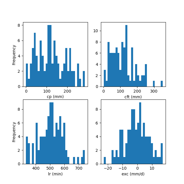
Note that if the mean value is too close to the bounds of the distribution, we use a truncated Gaussian distribution to generate samples, ensuring that they do not exceed their bounds. The distribution of generated samples can be visualized as shown below:

In [11]: f, ax = plt.subplots(2, 2, figsize=(6.4, 6.4))

In [12]: ax[0, 0].hist(sr.cp, bins=30);

In [13]: ax[0, 0].set_xlabel("cp (mm)");

In [14]: ax[0, 0].set_ylabel("Frequency");

In [15]: ax[0, 1].hist(sr.cft, bins=30);

In [16]: ax[0, 1].set_xlabel("cft (mm)");

In [17]: ax[1, 0].hist(sr.lr, bins=30, label="lr");

In [18]: ax[1, 0].set_xlabel("lr (min)");

In [19]: ax[1, 0].set_ylabel("Frequency");

In [20]: ax[1, 1].hist(sr.exc, bins=30, label="lr");

In [21]: ax[1, 1].set_xlabel("exc (mm/d)");

HDBC (High Dimensional Bayesian Calibration)

Once the samples are created in the sr object, we can employ an HDBC approach that incoporates multiple calibrations with VDA (using the \(\mathrm{L}\text{-}\mathrm{BFGS}\text{-}\mathrm{B}\) algorithm) and Bayesian estimation in high dimension. It can be implemented using the smash.Model.bayes_optimize method as follows:

In [22]: model_bo, br = model.bayes_optimize(
   ....:         sr,
   ....:         alpha=np.linspace(-1, 16, 60),
   ....:         mapping="distributed",
   ....:         algorithm="l-bfgs-b",
   ....:         options={"maxiter": 4},
   ....:         return_br=True
   ....:     )
   ....: 

In [23]: model_bo.output.cost  # cost value with HDBC
Out[23]: 0.1391131579875946

Note

In real-world applications, the maximum allowed number of iterations options["maxiter"] can be much larger to attain more accurate results.

Visualization of results

To visualize information about the Bayesian estimation process, we can use the br instance of smash.BayesResult. For instance, to display the histogram of the cost values when calibrating the Model parameters using the generated samples:

In [24]: plt.hist(br.data["cost"], bins=30, zorder=2);

In [25]: plt.grid(alpha=.7, ls="--", zorder=1);

In [26]: plt.xlabel("Cost");

In [27]: plt.ylabel("Frequency");

In [28]: plt.title("Cost value histogram for parameter set");

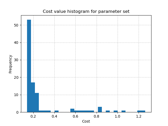
The minimal cost value through multiple calibrations:

In [29]: np.min(br.data["cost"])
Out[29]: 0.14008885622024536

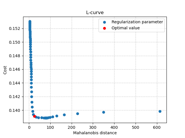
Then, can also visualize the L-curve that was used to find the optimal regularization parameter:

In [30]: opt_ind = np.where(br.lcurve["alpha"]==br.lcurve["alpha_opt"])[0][0]

In [31]: plt.scatter(
   ....:         br.lcurve["mahal_dist"],
   ....:         br.lcurve["cost"],
   ....:         label="Regularization parameter",
   ....:         zorder=2
   ....:     );
   ....: 

In [32]: plt.scatter(
   ....:         br.lcurve["mahal_dist"][opt_ind],
   ....:         br.lcurve["cost"][opt_ind],
   ....:         color="red",
   ....:         label="Optimal value",
   ....:         zorder=3
   ....:     );
   ....: 

In [33]: plt.grid(alpha=.7, ls="--", zorder=1);

In [34]: plt.xlabel("Mahalanobis distance");

In [35]: plt.ylabel("Cost");

In [36]: plt.title("L-curve");

In [37]: plt.legend();

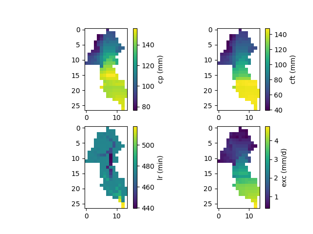
Finally, the spatially distributed model parameters can be visualized using the model_bo object:

In [38]: ma = (model_bo.mesh.active_cell == 0)

In [39]: ma_cp = np.where(ma, np.nan, model_bo.parameters.cp)

In [40]: ma_cft = np.where(ma, np.nan, model_bo.parameters.cft)

In [41]: ma_lr = np.where(ma, np.nan, model_bo.parameters.lr)

In [42]: ma_exc = np.where(ma, np.nan, model_bo.parameters.exc)

In [43]: f, ax = plt.subplots(2, 2)

In [44]: map_cp = ax[0,0].imshow(ma_cp);

In [45]: f.colorbar(map_cp, ax=ax[0,0], label="cp (mm)");

In [46]: map_cft = ax[0,1].imshow(ma_cft);

In [47]: f.colorbar(map_cft, ax=ax[0,1], label="cft (mm)");

In [48]: map_lr = ax[1,0].imshow(ma_lr);

In [49]: f.colorbar(map_lr, ax=ax[1,0], label="lr (min)");

In [50]: map_exc = ax[1,1].imshow(ma_exc);

In [51]: f.colorbar(map_exc, ax=ax[1,1], label="exc (mm/d)");