Pre-regionalization using artificial neural network#
Here, we aim to employ some physiographic descriptors to find the pre-regionalization mapping using an artificial neural network. Six descriptors are considered in this example, which are:
Slope
Drainage density
Karst
Woodland
Urban
Soil water storage
First, open a Python interface:
python3
Imports#
In [1]: import smash

In [2]: import matplotlib.pyplot as plt

In [3]: import numpy as np
Model object creation#
To perform the calibrations, you need to create a smash.Model object.
For this case, we will use the Lez dataset.
Load the setup and mesh dictionaries using the smash.load_dataset() method and create the smash.Model object.
In [4]: setup, mesh = smash.load_dataset("Lez")

In [5]: model = smash.Model(setup, mesh)
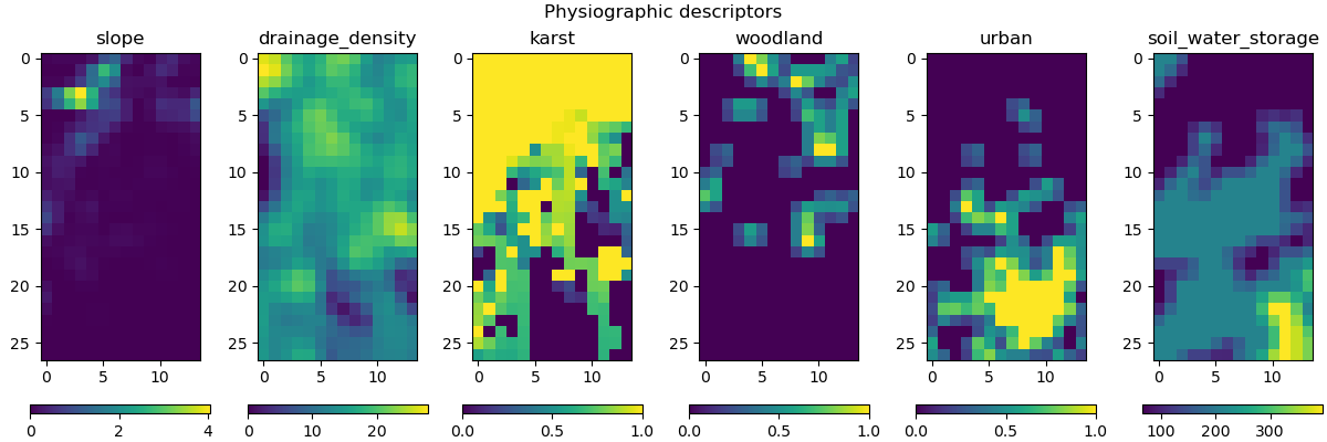
Visualization of descriptors#
This method requires input descriptors, which were provided during the creation of the Model object. We can visualize these descriptors and verify if they were successfully loaded:
In [6]: model.input_data.descriptor.shape
Out[6]: (27, 14, 6)
In [7]: desc_name = model.setup.descriptor_name

In [8]: fig, axes = plt.subplots(1, len(desc_name), figsize=(12,4), constrained_layout=True)

In [9]: for i, ax in enumerate(axes):
   ...:     ax.set_title(desc_name[i]);
   ...:     im = ax.imshow(model.input_data.descriptor[..., i]);
   ...:     cbar = fig.colorbar(im, ax=ax, orientation="horizontal");
   ...:     cbar.ax.tick_params();
   ...:

In [10]: fig.suptitle("Physiographic descriptors");
Defining the neural network#
If you do not specify the neural network (net argument) in the smash.Model.ann_optimize() method,
a default network will be used to learn the descriptors-to-parameters mapping.
This example shows how to define a custom neural network using the smash.Net() method.
To define a custom neural network, you may need to have information about the physiographic descriptors and hydrological parameters. This information will be used to determine the input and output layers of the network, including the number of descriptors, the control vector, and the boundary condition (if you want to scale the network output to the boundary condition). The default values of these parameters can be obtained as follows:
In [11]: problem = model.get_bound_constraints()

In [12]: problem
Out[12]:
{'num_vars': 4,
 'names': ['cp', 'cft', 'exc', 'lr'],
 'bounds': [[9.999999974752427e-07, 1000.0],
  [9.999999974752427e-07, 1000.0],
  [-50.0, 50.0],
  [9.999999974752427e-07, 1000.0]]}
In [13]: ncv = problem["num_vars"]  # number of control vector

In [14]: cv = problem["names"]  # control vector

In [15]: bc = problem["bounds"]  # default boundary condition

In [16]: nd = model.input_data.descriptor.shape[-1]  # number of descriptors
Next, we need to initialize the Net object:
In [17]: net = smash.Net()
Then, we can define a graph for our custom neural network by specifying the number of layers, type of activation function,
and output scaling. For example, we can define a neural network with 2 hidden dense layers followed by ReLU activation functions
and a final layer followed by a sigmoid function. To scale the network output to the boundary condition,
we apply a MinMaxScale function:
In [18]: net.add(layer="dense", options={"input_shape": (nd,), "neurons": 48})

In [19]: net.add(layer="activation", options={"name": "ReLU"})

In [20]: net.add(layer="dense", options={"neurons": 16})

In [21]: net.add(layer="activation", options={"name": "ReLU"})

In [22]: net.add(layer="dense", options={"neurons": ncv})

In [23]: net.add(layer="activation", options={"name": "sigmoid"})

In [24]: net.add(layer="scale", options={"bounds": bc})
Make sure to compile the network after defining it. We can also specify the optimizer and its hyperparameters:
In [25]: net.compile(optimizer="Adam", random_state=23, options={"learning_rate": 0.004})

In [26]: net  # display a summary of the network
Out[26]:
+----------------------------------------------------------+
| Layer Type            Input/Output Shape  Num Parameters |
+----------------------------------------------------------+
| Dense                 (6,)/(48,)          336            |
| Activation (ReLU)     (48,)/(48,)         0              |
| Dense                 (48,)/(16,)         784            |
| Activation (ReLU)     (16,)/(16,)         0              |
| Dense                 (16,)/(4,)          68             |
| Activation (Sigmoid)  (4,)/(4,)           0              |
| Scale (MinMaxScale)   (4,)/(4,)           0              |
+----------------------------------------------------------+
Total parameters: 1188
Trainable parameters: 1188
Optimizer: (adam, lr=0.004)
Training the neural network#
Now, we can train the neural network with the custom graph using the smash.Model.ann_optimize() method.
This method performs operation in-place on net:
In [27]: model_ann = model.ann_optimize(
   ....:         net,
   ....:         epochs=100,
   ....:         control_vector=cv,
   ....:         bounds=dict(zip(cv, bc))
   ....:     )
   ....:
Some information are also provided during the training process:
</> ANN Optimize Model
    Mapping: 'ANN' k(x) = N(D1, ..., Dn)
    Optimizer: adam
    Learning rate: 0.004
    Jobs function: [ nse ]
    wJobs: [ 1.0 ]
    Nx: 172
    Np: 52 [ cp cft exc lr ]
    Ns: 0 [  ]
    Ng: 1 [ Y3204040 ]
    wg: 1 [ 1.0 ]

    At epoch      1    J =  1.108795    |proj g| =  0.000060
    At epoch      2    J =  1.092934    |proj g| =  0.000062
    At epoch      3    J =  1.068635    |proj g| =  0.000062
    At epoch      4    J =  1.036452    |proj g| =  0.000060
    At epoch      5    J =  0.996259    |proj g| =  0.000057
    At epoch      6    J =  0.943647    |proj g| =  0.000051
    At epoch      7    J =  0.875171    |proj g| =  0.000067
    At epoch      8    J =  0.796573    |proj g| =  0.000132
    At epoch      9    J =  0.711945    |proj g| =  0.000190
    At epoch     10    J =  0.622793    |proj g| =  0.000198
    At epoch     11    J =  0.536326    |proj g| =  0.000148
    At epoch     12    J =  0.465874    |proj g| =  0.000075
...
    At epoch     98    J =  0.136344    |proj g| =  0.000023
    At epoch     99    J =  0.136195    |proj g| =  0.000023
    At epoch    100    J =  0.136045    |proj g| =  0.000020
Training: 100%|███████████████████████████████| 100/100 [00:03<00:00, 26.63it/s]
Note
To ensure the order of the control vectors and to prevent any potential conflicts, it is recommended that you redefine
the control_vector and bounds arguments in the smash.Model.ann_optimize() function as the code above.
Visualization of results#
To visualize the descent of the cost function, we use the net object and create a plot of the cost function value versus
the number of iterations. Here’s an example:
In [28]: y = net.history["loss_train"]

In [29]: x = range(1, len(y) + 1)

In [30]: plt.plot(x, y);

In [31]: plt.xlabel("Epoch");

In [32]: plt.ylabel("$1-NSE$");

In [33]: plt.grid(alpha=.7, ls="--");

In [34]: plt.title("Cost funciton descent");
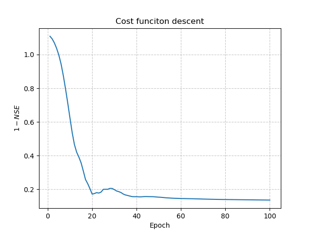
Note
By default, nse is used to define the objective function if you do not specify the jobs_fun argument
in smash.Model.ann_optimize().
The simulated discharge:
In [35]: qo = model_ann.input_data.qobs[0,:].copy()

In [36]: qo = np.where(qo<0, np.nan, qo)  # to deal with missing data

In [37]: plt.plot(qo, label="Observed discharge");

In [38]: plt.plot(model_ann.output.qsim[0,:], label="Simulated discharge");

In [39]: plt.grid(alpha=.7, ls="--");

In [40]: plt.xlabel("Time step");

In [41]: plt.ylabel("Discharge $(m^3/s)$");

In [42]: plt.title(model_ann.mesh.code[0]);

In [43]: plt.legend();

The cost value:
In [44]: model_ann.output.cost
Out[44]: 0.13604475557804108
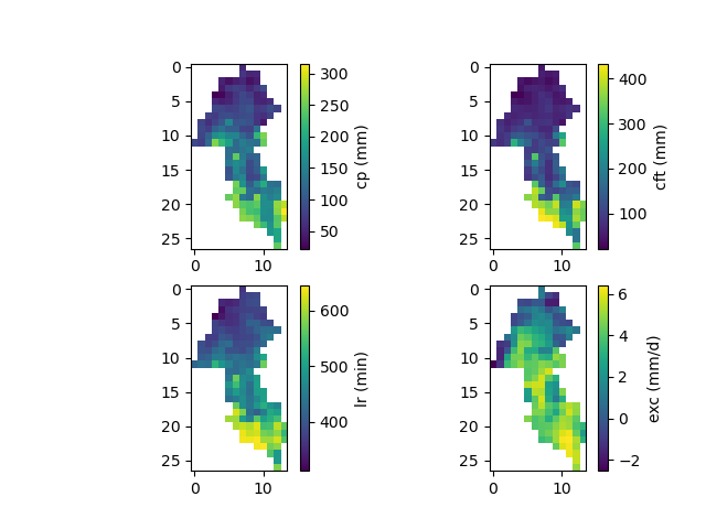
And finally, the spatially distributed model parameters constrained by physiographic descriptors:
In [45]: ma = (model_ann.mesh.active_cell == 0)

In [46]: ma_cp = np.where(ma, np.nan, model_ann.parameters.cp)

In [47]: ma_cft = np.where(ma, np.nan, model_ann.parameters.cft)

In [48]: ma_lr = np.where(ma, np.nan, model_ann.parameters.lr)

In [49]: ma_exc = np.where(ma, np.nan, model_ann.parameters.exc)

In [50]: f, ax = plt.subplots(2, 2)

In [51]: map_cp = ax[0,0].imshow(ma_cp);

In [52]: f.colorbar(map_cp, ax=ax[0,0], label="cp (mm)");

In [53]: map_cft = ax[0,1].imshow(ma_cft);

In [54]: f.colorbar(map_cft, ax=ax[0,1], label="cft (mm)");

In [55]: map_lr = ax[1,0].imshow(ma_lr);

In [56]: f.colorbar(map_lr, ax=ax[1,0], label="lr (min)");

In [57]: map_exc = ax[1,1].imshow(ma_exc);

In [58]: f.colorbar(map_exc, ax=ax[1,1], label="exc (mm/d)");